1  Getting Started with R

Welcome to Lab 1! In this first chapter, we’ll embark on an exciting journey into the world of R programming and the powerful RStudio Integrated Development Environment (IDE). Whether you’re new to programming or already familiar with other languages, this lab is designed to lay a solid foundation for your future explorations in data analysis and statistical computing.

By the end of this lab, you’ll have a strong grasp of the basics of R programming, setting you up to dive deeper into more complex topics later on.

Here’s what we’ll cover:

• Exploring the RStudio Interface
  You’ll get acquainted with the four main panes of RStudio and see how each one contributes to a smooth and efficient coding experience.

• Performing Basic Calculations
  You’ll learn how to use R as a calculator, performing arithmetic operations while understanding the order of operations.

• Understanding Atomic Data Types
  We’ll delve into the fundamental data types in R, such as numeric, character, and logical types, which are essential building blocks for working with data.

• Assigning Variables:
  You’ll practice creating variables, assigning values to them, and following proper naming conventions, an essential skill for organizing your code.

• Using Conditional Statements
  You’ll explore how to control the flow of your programs using if, else if, and else statements, along with logical operators, allowing your code to make decisions based on conditions.

By completing this lab, you’ll not only be comfortable with the RStudio environment but also able to perform basic calculations, manipulate data types, assign variables, and write simple scripts that make decisions based on conditions. This is your first step toward mastering R and unlocking its potential for data analysis and statistical computing.

1.1 Introduction

R is a powerful programming language and software environment used extensively for statistical computations, data cleaning, data analysis, and graphical representation of data. It’s a vital tool for statisticians, data scientists, and anyone interested in data mining. Since its inception, R has become a cornerstone in the field of data analysis, celebrated for its versatility and community support.

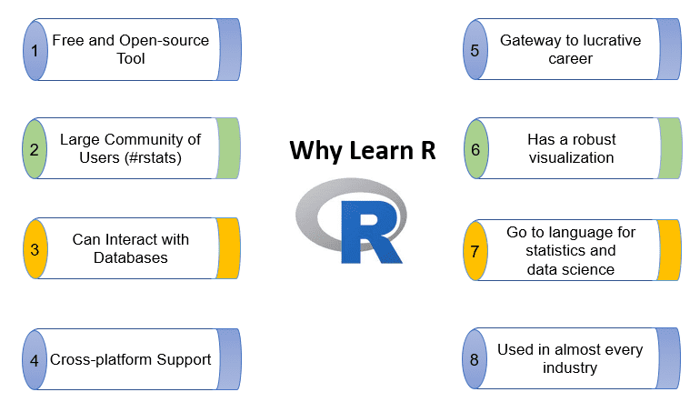
1.1.1 Why learning R programming?

Learning R opens doors to a vast ecosystem of packages and resources that make data analysis and visualization more accessible and efficient. Its active community continually contributes to its development, ensuring that it stays up-to-date with the latest methodologies in data science.

Figure 1.1: Compelling Reasons to Learn R

1.1.2 Companies Using R for Analytics

Many leading companies leverage R for their analytics needs, demonstrating its practical applications in the industry. You can find a list of such companies here.

Figure 1.2: Major Companies Using R Programming

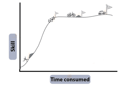
1.1.3 Learning Curve

While R might seem challenging at first, many users find that it simplifies complex tasks once you get the hang of it. Think of it as making difficult things easy and easy things even easier!

Figure 1.3: The Learning Curve of R Programming

1.1.4 Installing R and RStudio

Before we dive in, you’ll need to have both R and RStudio installed on your computer. R is the core programming language, while RStudio provides a user-friendly interface that enhances your coding experience.

Figure 1.4: Overview of the RStudio Interface

Installing R

The installation process for R varies slightly depending on your operating system:

• For Windows Users:

  Visit the CRAN (Comprehensive R Archive Network) website at this link. Download the latest version of R for Windows, then follow the installation prompts to complete the setup.

• For Mac Users:

  Head over to the CRAN website for Mac at this link. Download the appropriate version for your macOS, and follow the on-screen instructions to install it.

Installing RStudio

Once R is installed, you’ll want to install RStudio, which provides an easier interface to interact with R.

• Visit the RStudio download page. Select the free version of RStudio Desktop, and download the appropriate installer for your operating system (Windows, macOS, or Linux). Then, run the installer and follow the instructions.

With both R and RStudio installed, you’re ready to start your journey into data analysis, statistical computing, and programming with R!

1.2 Experiment 1.1: RStudio Interface and Basic Calculations

In this experiment, you will begin working with R. You will learn how to navigate the four panes in RStudio, use R as a calculator, assign values to variables, and understand basic data types.

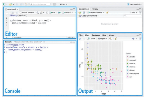
1.2.1 The Four Panes of RStudio

RStudio is divided into four main panes, each serving a specific purpose to enhance your coding workflow¹.

Figure 1.5: Annotated Overview of Key RStudio Panels

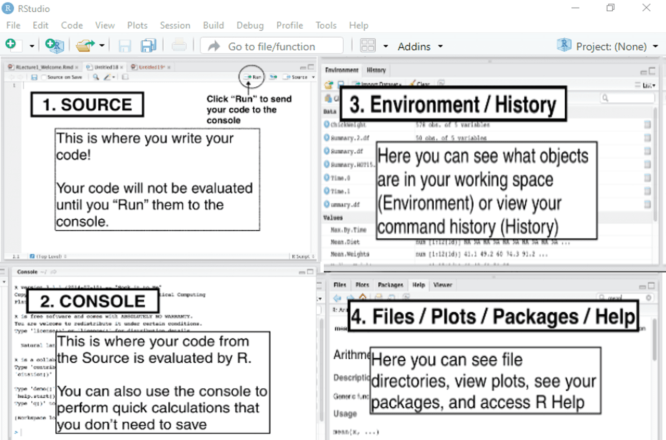
Source Pane

• This is where you write your R code. Think of it as your notepad or a place to draft your work.

• The code you write here won’t run until you specifically tell it to. You do this by clicking the “Run” button or using the keyboard shortcut (Ctrl + Enter for Windows or Cmd + Enter for Mac).

• The Source Pane is great for writing scripts that you can save and use later.

Console Pane

• This is the heart of R’s interaction with you. It’s where R evaluates your commands.

• When you “Run” your code from the Source, it shows up here, and R processes it immediately.

• You can also directly type commands here for quick calculations or testing. However, anything you type in the console won’t be saved if you close RStudio.

Environment/History Pane

• Environment Tab: This shows you all the variables, data frames, and objects you’ve created in your current R session. It’s like a snapshot of everything you’re working with.

• History Tab: This keeps a record of every command you’ve entered, allowing you to track what you’ve done so far.

Files/Plots/Packages/Help Pane

• Files Tab: View and manage the files on your computer, similar to a file explorer.

• Plots Tab: Displays any graphs or charts you create with your R code.

• Packages Tab: Shows the packages (additional tools and functions) available in R and allows you to install, load, or update them as needed.

• Help Tab: This is your go-to place for understanding how functions work. If you’re unsure about something, R’s built-in documentation will be here to guide you.

1.2.2 Basic Calculations in R Programming

R can perform all standard arithmetic operations, making it a handy calculator.

Figure 1.6: R Programming as a Powerful Calculator

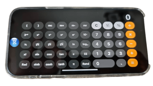
The basic operators include:

• Addition (+)

• Subtraction (-)

• Multiplication (*)

• Division (/)

• Exponentiation (^)

• Modulo (%%)

• Parenthesis ()

Arithmetic Operations

6 + 12 - 8

#> [1] 10

2 * 3

#> [1] 6

100 / 50

#> [1] 2

3 * 5 / 3

#> [1] 5

3^2

#> [1] 9

Modulus

The modulo (or “modulus” or “mod”) is the remainder after division. For example, 9 mod 2 = 1. Because 9/2 = 4 with a remainder of 1. In mathematics, we write that as 9 mod 2 = 1 and in R we write it as 9 %% 2 = 1.

9 %% 2 # Returns 1

#> [1] 1

Parenthesis or brackets

Parentheses are used to denote grouping of operation in mathematics. It denotes modifications to normal order of operations. Do you remember BODMAS in mathematics? We shall use BEDMAS: Brackets, Exponentiation, Division, Multiplication, Addition, Subtraction in programming.

In an expression like \(3 \times (2+3)\), the part of the expression within the parentheses, \((2 + 3) = 5\), is evaluated first, and then this result is used in the rest of the expression i.e. \(3 \times 5 = 15\).

3 * (2 + 3) # Returns 15

#> [1] 15

(3 + 2) * (6 - 4) # Returns 10

#> [1] 10

Operations Involving Square Roots

To calculate square roots, use the sqrt() function.

\(\sqrt{125}\)

sqrt(125)

#> [1] 11.18034

\(\dfrac{19}{\sqrt{19}}\)

19 / sqrt(19)

#> [1] 4.358899

1.2.3 Comments in R

Comments are lines in your code that R ignores during execution. They are marked by the # symbol and are essential for:

1. Understanding your code later.

2. Helping others understand your code.

3. Documentation purposes.

Example:

# Multiplying 2 by 8

2 * 8

#> [1] 16

It’s good practice to add a space after the # for readability.

3 + 6 # Adding 3 and 6

#> [1] 9

1.2.4 Comparison Operators

Comparison operators compare values and return TRUE or FALSE, known as logical. The following are the most common comparison operators in R:

• Equal to (==)

• Not equal to (!=)

• Greater than (>)

• Less than (<)

• Greater than or equal to (>=)

• Less than or equal to (<=)

5 == 3 # Returns FALSE

#> [1] FALSE

25 != 10 # Returns TRUE

#> [1] TRUE

100 > 30 # Returns TRUE

#> [1] TRUE

60 >= 45 # Returns TRUE

#> [1] TRUE

100 <= 1000 # Returns TRUE

#> [1] TRUE

1.2.5 Exercise 1.1.1

• Explore RStudio: Open RStudio and familiarize yourself with the four panes.

• Perform Calculations: In the Source Pane, compute the following, adding comments where appropriate:

  • \(2 + 6 -12\)

  • \(4 \times 3 - 8\)

  • \(81\div 6\)

  • \(16 \text{ mod } 3\)

  • \(2^3\)

  • \((3 + 2) \times (6 - 4) + 2\)

1.3 Experiment 1.2: Atomic Data Type and Variable Assignment in R

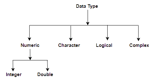
R works with several atomic data types:

• Numeric: Integers or doubles (e.g., 4, -2, 4.7, -0.26)

• Character: Text strings enclosed in quotes (e.g., "Nigeria", "Hello world")

• Logical: Boolean values (TRUE, FALSE)

Figure 1.7: Data Types in R Programming

You can determine the data type of an object using the class() function.

class(2) # Returns "numeric"

#> [1] "numeric"

class("Anthony Joshua") # Returns "character"

#> [1] "character"

class(TRUE) # Returns "logical"

#> [1] "logical"

1.3.1 Variable Assignment

When working in R, you’ll often find yourself storing values, results, or objects for later use. This is where variables come in. Variables allow you to hold onto data so that you can reference it easily whenever you need it. Assigning a value to a variable is straightforward in R, and you can do this using the assignment operator, which is <- or =. While both work, you’ll notice that most R users prefer <- for assignments. This preference is largely based on convention and readability, as it helps keep your code clean and consistent².

Let’s walk through a few examples to see variable assignment in action. Here, we’ll assign different types of data to variables.

number <- 10 # 'number' now holds the value 10

class(number) # Returns "numeric"

#> [1] "numeric"

state <- "Lagos"

class(state) # Returns "character"

#> [1] "character"

After running these lines, each variable (number, state) stores a value that you can reuse or modify later in your code. For instance, if you want to check the value of number, just type:

number

#> [1] 10

… and R will display the stored value.

Tip

If you’re using a Windows, a quick way to type the assignment operator <- is by pressing ALT + _, while on a Mac, you can use Option + _. This shortcut can save you time as you write and assign variables in R.

Once you’ve assigned a value to a variable, you can use that variable in expressions. For instance:

x <- 15

y <- 12

x + 1

#> [1] 16

x + y

#> [1] 27

It’s also good to know that you can overwrite variables if needed. Say you assigned x <- 15, but later, you decide x should be 20. You can just assign it again:

x <- 20

Now, every time you call x, R will know that its value is 20, not 15 anymore.

1.3.2 Rules for Naming Variables

• Must start with a letter.

• Can contain letters, numbers, underscores _, or dots . after the first letter.

• No spaces or special characters.

• R is case-sensitive (Age and age are different variables).

Quick Tips

• Name Your Variables Clearly: Choose names that describe the data they hold, like total_sales or average_height, rather than generic names like x or y. Using clear, descriptive variable names is a best practice because it makes your code easier to understand and maintain. This way, anyone reading your code can quickly grasp the purpose of each variable without needing additional explanations.

• Avoid Overwriting R’s Built-in Functions: Names like mean, sum, and data are already used by R, so avoid using these as variable names to prevent errors.

In short, variable assignment is like giving a shortcut name to a value or a piece of data. Once assigned, you can call on that name whenever you need it, making your code easier to follow and maintain. And remember, R is pretty flexible, so don’t worry too much if you make a mistake – you can always reassign or update your variables as you go!

1.3.3 Exercise 1.2.1: Acceptable vs. Unacceptable Variable Names

In this exercise, you will explore the differences between acceptable and unacceptable variable names in R. Understanding why some naming conventions work and others don’t is essential for writing clean, error-free code.

Instructions:

1. Review the table below and identify why each name is either acceptable or unacceptable according to R’s variable naming rules.

2. Answer the following questions:

   • Why are some variable names acceptable while others are not?
   • What makes the acceptable variable names follow R’s rules and best practices?

3. Reflect on how these rules can help make your code more readable and easier to debug.

Table of Variable Names

Acceptable Variable Names	Unacceptable Variable Names
health.status	health(status)
covid_19_cases	covid-19-cases
budget2024	2024budget
sales_price_2024	sales price 2024

Discussion Questions

1. Periods and Underscores: Why are periods (.) and underscores (_) commonly used in acceptable variable names instead of symbols like hyphens or spaces?
2. Special Characters: What happens if you use special characters like parentheses (()) in a variable name? Why does R disallow these?
3. Starting with Letters: Why is it important to start a variable name with a letter rather than a number?

Reflect on these questions and write down your answers in a few sentences for each. Use these answers as a guide to create variable names that follow R’s rules and make your code easy to understand.

Comparison of Variable Naming Conventions
Acceptable vs. Unacceptable Variable Names
Acceptable Variable Names	Unacceptable Variable Names
health.status	health(status)
covid_19_cases	covid-19-cases
budget2024	2024budget
sales_price_2024	sales price 2024

1.3.4 Data Type Conversions

Sometimes you need to convert data from one type to another, known as typecasting. Use the as. functions. The following table shows examples of those functions:

Data Type Converting To	How to Do It
Numeric	as.numeric(variable_name)
Character	as.character(variable_name)
Logical	as.logical(variable_name)
Complex	as.complex(variable_name)

Data Type Conversion in R
Common Functions to Convert Between Data Types
Data Type Converting To	How to Do It
Numeric	as.numeric(variable_name)
Character	as.character(variable_name)
Logical	as.logical(variable_name)
Complex	as.complex(variable_name)

Suppose you have:

weight <- "64.45"

class(weight) # Returns "character"

#> [1] "character"

Convert weight to numeric:

weight_num <- as.numeric(weight)

class(weight_num) # Returns "numeric"

#> [1] "numeric"

Handling NA Results

If R can’t convert a value, it returns NA (Not Available). This often happens when:

• Converting a character string that contains letters or symbols to numeric.

• Converting non-boolean strings to logical.

height <- "161.5 cm"

as.numeric(`height`) # Returns NA with a warning

#> Warning: NAs introduced by coercion

#> [1] NA

smiling_face <- "No"

as.logical(`smiling_face`) # Returns NA

#> [1] NA

1.3.5 Exercise 1.2.2

Determine the classes of the following variables and convert them if necessary:

age <- 15

class(age) # What is the class?

#> [1] "numeric"

diabetic_status <- "No"

class(diabetic_status) # What is the class?

#> [1] "character"

five_less_than_2 <- FALSE

class(five_less_than_2) # What is the class?

#> [1] "logical"

weight <- "60.4 kg"

class(weight) # What is the class?

#> [1] "character"

# Can you convert weight to numeric?

smile_face <- "FALSE"

class(smile_face) # What is the class?

#> [1] "character"

# What happens if you convert smile_face to logical?

1.4 Experiment 1.3: Conditional Statements in R

Conditional statements allow your program to make decisions based on certain conditions. The primary constructs are if, else if, and else.

Figure 1.8: If-Else Statement in R Programming

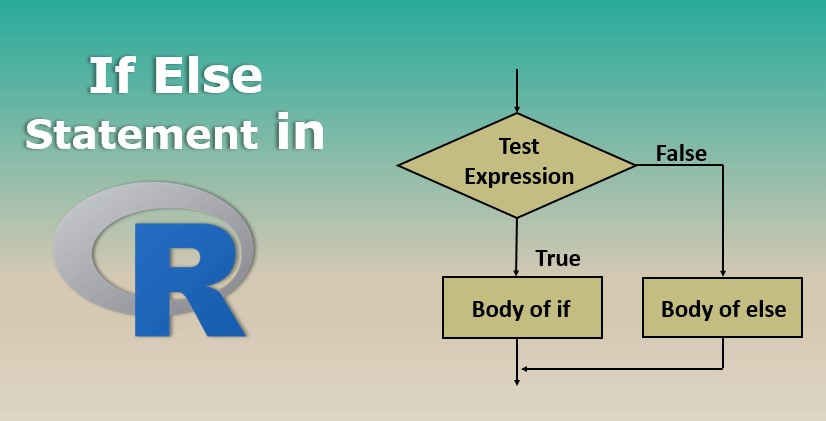
1.4.1 The if Statement

This is the most basic conditional construct. It executes code only if a specified condition is TRUE.

x <- 5
if (x > 3) {
  print("x is greater than 3")
}

#> [1] "x is greater than 3"

1.4.2 The else Statement

Provides an alternative set of instructions if the if condition is FALSE.

x <- 2
if (x > 3) {
  print("x is greater than 3")
} else {
  print("x is not greater than 3")
}

#> [1] "x is not greater than 3"

1.4.3 The else if Statement

For situations with multiple conditions to check sequentially, else if can be used. It provides an additional condition check after the initial if statement.

x <- 3
if (x > 5) {
  print("x is greater than 5")
} else if (x == 5) {
  print("x is equal to 5")
} else {
  print("x is less than 5")
}

#> [1] "x is less than 5"

Using Logical Operators

You can combine conditions using logical operators:

• AND (&)
• OR (|)
• NOT (!)

Example using AND (&):

x <- 8
y <- 12

if (x < 10 & y > 10) {
  print("Both conditions are true")
} else {
  print("At least one condition is false")
}

In this example, the if statement checks if both x < 10 and y > 10 are TRUE. Since both conditions are TRUE, the output will be:

"Both conditions are true"

Example using OR (|):

a <- 3
b <- 20

if (a < 5 | b > 25) {
  print("At least one condition is true")
} else {
  print("Neither condition is true")
}

In this example, the if statement checks if either a is less than 5 or b is greater than 25. Since a < 5 is TRUE, the output will be: 

"At least one condition is true"

Example using NOT (!):

c <- FALSE

if (!c) {
  print("The condition is false")
} else {
  print("The condition is true")
}

Here, the if statement uses the NOT operator to check if c is not TRUE. Since c is FALSE, !c becomes TRUE, and the output will be:

"The condition is false"

1.4.4 The switch function

The switch() function is a control flow statement that allows you to execute different pieces of code based on the value of an expression. It’s particularly useful when you have multiple conditions to check and want a cleaner alternative to lengthy if...else statements.

There are two primary ways to use switch() in R:

1. Numeric Switching: Where the expression evaluates to a numeric index.

2. Character Switching: Where the expression evaluates to a character string matching one of the named alternatives.

The general structure of switch() function is as follows:

switch(EXPR,
  ...
)

where:

• EXPR: An expression that evaluates to a numeric value or a character string.

• ...: A sequence of alternatives (unnamed or named arguments).

The switch() function uses the same syntax for both numeric and character expressions. The behavior of the function depends on the type of the EXPR argument you provide.

When to Use switch()

• When you have a variable that can take on multiple known values and you want to execute different code based on each value.

• To improve code readability over multiple if...else statements.

• When performance is a consideration, as switch() can be more efficient than multiple if...else checks.

1.4.4.1 Example: Day of the Week Activities Using Character Switching

Suppose you want to plan activities based on the day of the week.

day <- "Saturday"

activity <- switch(day,
  Monday = "Go to the gym",
  Tuesday = "Attend a cooking class",
  Wednesday = "Work from home",
  Thursday = "Meet friends for dinner",
  Friday = "Watch a movie",
  Saturday = "Go hiking",
  Sunday = "Rest and recharge",
  "Invalid day"
)

print(paste("Today's activity:", activity))

#> [1] "Today's activity: Go hiking"

Explanation

• Variable day: Contains the day of the week as a string.

• Using switch():

  • Matches day against the provided day names.

  • If a match is found, returns the corresponding activity.

  • If no match is found, returns "Invalid day".

1.4.4.2 Example: Mapping Codes to Descriptions Using Character Switching

Suppose you have status codes that need to be mapped to descriptive messages.

status_code <- 404

message <- switch(as.character(status_code),
  "200" = "OK: The request has succeeded.",
  "301" = "Moved Permanently: The resource has moved.",
  "400" = "Bad Request: The request could not be understood.",
  "401" = "Unauthorized: Authentication is required.",
  "404" = "Not Found: The resource could not be found.",
  "500" = "Internal Server Error: The server encountered an error.",
  "Unknown Status Code"
)

print(message)

#> [1] "Not Found: The resource could not be found."

Explanation:

• Variable status_code: Contains an HTTP status code.

• Converting to Character: as.character(status_code) because switch() with character matching requires a string.

• Using switch():

  • Matches the status code against the provided cases.

  • Returns the corresponding message or "Unknown Status Code" if no match is found.

1.4.4.3 Example: Simple Calculator Using Numeric Switching

Let’s create a simple calculator that performs operations based on a numeric choice.

# User inputs
num1 <- 10
num2 <- 5
choice <- 3 # Options: 1 for addition, 2 for subtraction, 3 for multiplication, 4 for division

# Use switch() to perform the selected operation
result <- switch(choice,
  num1 + num2, # If choice == 1
  num1 - num2, # If choice == 2
  num1 * num2, # If choice == 3
  if (num2 != 0) num1 / num2 else "Division by zero error", # If choice == 4
  "Invalid operation"
) # Default if choice > number of cases

# Display the result
print(paste("The result is:", result))

#> [1] "The result is: 50"

Explanation

• Variables:

  • num1, num2: Numbers to operate on.

  • choice: Numeric choice of operation.

• Using switch():

  • Since choice is numeric, switch() selects the expression based on position.

    • 1: num1 + num2

    • 2: num1 - num2

    • 3: num1 * num2

    • 4: Division with a check for division by zero.

  • If choice exceeds the number of provided alternatives (4), the default "Invalid operation" is returned.

1.4.5 Exercise 1.3.1

Task 1

What is the output of the following code?

a <- 10
if (a %% 2 == 0) {
  print("Even")
} else {
  print("Odd")
}

#> [1] "Even"

Task 2

Given m <- 5 and n <- 7, write code that prints:

• “m is greater than n” if m > n
• “m is less than n” if m < n
• “m and n are equal” if m == n

1.4.6 Exercise 1.3.2: Menu Selection Using switch()

Simulate a simple text-based menu where a user selects an option. Use the switch() function to determine the action based on the user’s selection.

Your Task:

1. Simulate User Input:

   • Assign a value to a variable option to represent the user’s selection.

   • Possible options: "balance", "deposit", "withdraw", "exit".

2. Use the switch() Function:

   • Match the value of option to the appropriate case using switch().

   • For each case, assign a message that describes the action.

Possible Options and Messages:

• “balance”: Display “Your current balance is $1,000.”

• “deposit”: Display “Enter the amount you wish to deposit.”

• “withdraw”: Display “Enter the amount you wish to withdraw.”

• “exit”: Display “Thank you for using our banking services.”

• Default: Display “Invalid selection. Please choose a valid option.”

3. Include a Default Case:
   • If the user input does not match any of the specified options, provide a default message indicating an invalid selection.
4. Display the Message:
   • Use print() to display the message corresponding to the user’s selection.

Here’s a starting point for your code:

# Simulate user input
option <- "---" # Options could be "balance", "deposit", "withdraw", "exit"

# Use switch() to determine the action
message <- switch(...,
  balance = "You have $1,000 in your account.",
  deposit = ...,
  withdraw = "How much would you like to withdraw?",
  "Invalid selection. Please choose a valid option."
)

# Display the message
print(...)

Replace the ... with the correct values and complete the exercise!

1.5 Additional R Learning Resources

To further enhance your R programming skills, here are some excellent resources:

• YaRrr! The Pirate’s Guide to R by Nathaniel D. Phillips

• R for Data Science by Hadley Wickham, Mine Çetinkaya-Rundel, and Garrett Grolemund.

• R for Data Science: Exercise Solutions by Jeffrey B. Arnold

• Big Book of R by Oscar Baruffa

• Posts you might have missed!

1.6 Summary

Congratulations on completing Lab 1! You’ve taken your first steps into R programming and have covered a lot of ground:

• Navigating the RStudio Interface
  You learned how to use RStudio’s four main panes to write, execute, and manage your R code effectively.

• Performing Basic Calculations
  You practiced using R for arithmetic operations, understood operator precedence, and learned how to use mathematical functions.

• Understanding Atomic Data Types
  You explored numeric, character, and logical data types, and learned how to identify and convert between them.

• Assigning Variables
  You mastered variable assignment, followed naming conventions, and performed operations using variables.

• Constructing Conditional Statements
  You learned how to control the flow of your programs using if, else if, and else statements, and how to use logical operators.

As you move forward in this book, these foundational skills will be invaluable. In the next lab, we’ll delve into R’s basic data structures, such as vectors, matrices, and data frames, which are essential for data manipulation and analysis.

Keep practicing, and don’t hesitate to revisit this lab if you need a refresher. Happy coding!

---

1. For a detailed overview of all RStudio’s features, see the RStudio User Guide at https://docs.posit.co/ide/user.

2. You might wonder why R uses <- instead of the = symbol that you might see in other programming languages. While you can use = for assignment in R, it’s generally preferred to use <- for clarity. This is partly because = is also used in function arguments, so sticking to <- makes your code easier to read and helps avoid confusion.