4  Managing Packages & Workflows

In this Lab 4, we will explore essential practices that will enhance your efficiency and effectiveness as an R programmer. You’ll learn how to extend R’s capabilities by installing and loading packages, ensure that your analyses are reproducible using RStudio Projects, proficiently import and export datasets in various formats, and handle missing data responsibly. These skills are crucial for any data analyst or data scientist, as they enable you to work with a wide range of data sources, maintain the integrity of your analyses, and share your work with others in a consistent and reliable manner.

By the end of this lab, you will be able to:

• Install and Load Packages in R
  Learn how to find, install, and load packages from CRAN and other repositories to extend the functionality of R for your data analysis tasks.

• Ensure Reproducibility with R and RStudio Projects
  Set up and manage RStudio Projects to organize your work, understand the concept of the working directory, and adopt best practices to make your data analyses reproducible and shareable.

• Import and Export Datasets of Various Formats
  Import data into R from different file types such as CSV, Excel, SPSS, and more, using appropriate packages and functions. Export your data frames and analysis results to various formats for sharing or reporting.

• Handle and Impute Missing Data
  Identify missing values in your datasets, understand how they can impact your analyses, and apply appropriate techniques to handle and impute missing data effectively.

By completing Lab 4, you’ll enhance your ability to manage and analyze data in R efficiently, ensuring that your work is organized, reproducible, and ready to share with others. These foundational skills will support your growth as a proficient R programmer and data analyst.

4.1 Introduction

In R, a package is a collection of functions, data, and compiled code that extends the basic functionality of R. Think of it as a toolkit for specific tasks or topics. For example, packages like tidyr and janitor are designed for data wrangling.

The place where these packages are stored on your computer is called a library. When you install a package, it gets saved in your library, making it easily accessible when needed.

4.2 Compiling R Packages from Source

To work effectively with packages in R, especially when compiling from source, certain tools are necessary depending on your operating system.

• Windows: Rtools is a collection of software needed to build R packages from source, including a compiler and essential libraries. Since Windows does not natively support code compilation, Rtools provides these capabilities. You can download Rtools from CRAN: https://cran.rstudio.com/bin/windows/Rtools/. After downloading and installing the version of Rtools that matches your R version, R will automatically detect it.

Note

To check your R version, run the following code in the console:

R.version

• Mac OS: Unlike Windows, Mac OS users need the Xcode Command Line Tools, which provide similar compiling capabilities as Rtools. These tools include necessary libraries and compilers. You can install Xcode from the Mac App Store: http://itunes.apple.com/us/app/xcode/id497799835?mt=12 or install the Command Line Tools directly by entering:

xcode-select --install

• Linux: Most Linux distributions already come with the necessary tools for compiling packages. If additional developer tools are needed, you can install them via your package manager, usually by installing packages like build-essential or similar for your Linux distribution.

Note

On Debian/Ubuntu, you can install the essential software for R package development and LaTeX (if needed for documentation) with:

sudo apt-get install r-base-dev texlive-full

To ensure all dependencies for building R itself from source are met, you can run:

sudo apt-get build-dep r-base-core

4.3 Experiment 4.1: Installing and Loading Packages

As you work in R, you’ll often need additional functions that aren’t included in the base installation. These come in the form of packages, which you can easily install and load into your R environment.

4.3.1 Installing Packages from CRAN

The Comprehensive R Archive Network (CRAN) hosts thousands of packages. To install a package from CRAN, use install.packages():

install.packages("package_name")

Note

Replace package_name with the name of the package you want to install.

For example, to install the tidyverse package, use:

install.packages("tidyverse")

Similarly, to install the janitor package, use:

install.packages("janitor")

Warning

Remember to enclose the package name in quotes—either double ("package_name") or single ('package_name').

4.3.2 Installing Packages from External Repositories

Packages not available on CRAN can be installed from external sources like GitHub. First, install a helper package like devtools or remotes:

install.packages("devtools")
# or
install.packages("remotes")

Then, to install a package from GitHub, for example fakir package, use:

devtools::install_github("ThinkR-open/fakir")
# or
remotes::install_github("ThinkR-open/fakir")

You can also install development versions of packages using these helper packages. For instance:

remotes::install_github("datalorax/equatiomatic")

4.3.3 Loading Installed Packages

Once a package has been installed, you need to load it into your R session to use its functions. You can do this by calling the library() function, as demonstrated in the code cell below:

library(package_name)

Here, package_name refers to the specific package you want to load into the R environment. For example, to load the tidyverse package:

library(tidyverse)

#> ── Attaching core tidyverse packages ──────────────────────── tidyverse 2.0.0 ──
#> ✔ dplyr     1.1.4     ✔ readr     2.1.5
#> ✔ forcats   1.0.0     ✔ stringr   1.5.1
#> ✔ ggplot2   3.5.1     ✔ tibble    3.2.1
#> ✔ lubridate 1.9.3     ✔ tidyr     1.3.1
#> ✔ purrr     1.0.2     
#> ── Conflicts ────────────────────────────────────────── tidyverse_conflicts() ──
#> ✖ dplyr::filter() masks stats::filter()
#> ✖ dplyr::lag()    masks stats::lag()
#> ℹ Use the conflicted package (<http://conflicted.r-lib.org/>) to force all conflicts to become errors

Executing this single line of code loads the core tidyverse packages, which are essential tools for almost every data analysis project¹.

Other installed packages can also be loaded in such manner:

library(janitor)

#> 
#> Attaching package: 'janitor'

#> The following objects are masked from 'package:stats':
#> 
#>     chisq.test, fisher.test

library(bulkreadr)

#> Welcome to bulkreadr package! To learn more, please run:
#> browseURL("https://gbganalyst.github.io/bulkreadr")
#> to visit the package website.

#> 
#> Attaching package: 'bulkreadr'

#> The following object is masked from 'package:janitor':
#> 
#>     convert_to_date

If you run this code and get the error message there is no package called "bulkreadr", you’ll need to first install it, then run library() once again.

install.packages("bulkreadr")

library(bulkreadr)

Tip

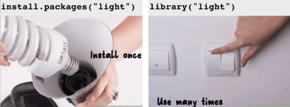
You only need to install a package once, but you must load it each time you start a new R session.

Figure 4.1: Installing vs. Loading Packages in R

4.3.4 Using Functions from a Package

There are two main ways to call a function from a package:

1. Load the package and call the function directly:

library(janitor)

clean_names(data_frame)

2. Use the :: operator to call a function without loading the package:

janitor::clean_names(data_frame)

Tip

Using package::function() is helpful because it makes your code clearer about where the function comes from, especially if multiple packages have functions with the same name.

Example:

Let’s see how to load a package and use one of its functions. We’ll use the clean_names() function from the janitor package to clean column names in a data frame.

library(janitor)

Now, let’s clean the column names of iris data frame:

clean_names(iris)

Example:

Using a function without loading the package:

janitor::clean_names(iris)

4.4 Experiment 4.2: Data Analysis Reproducibility with R and RStudio Projects

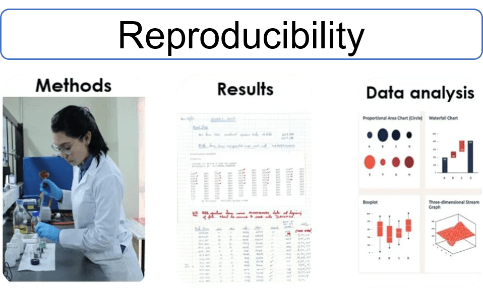
Reproducibility is vital in data analysis. Using RStudio Projects helps you organize your work and ensures that your analyses can be easily replicated.

Figure 4.2: Key Aspects of Reproducibility in Research

4.4.1 Where Does Your Analysis Live?

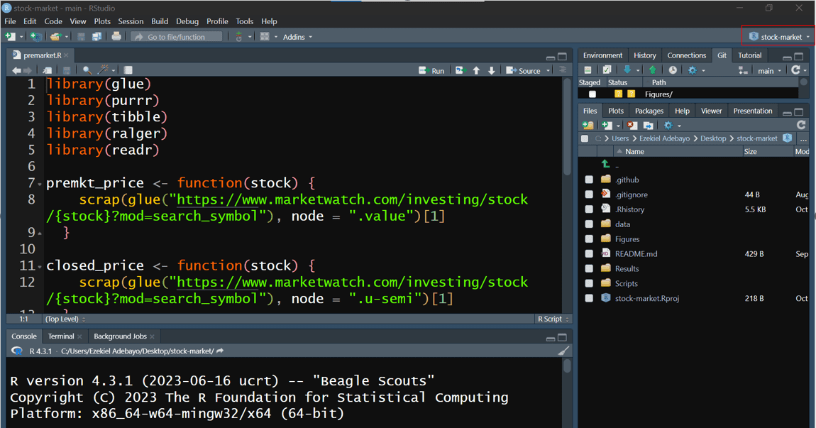
The working directory is where R looks for files to load and where it saves output files. You can see your current working directory at the top of the console:

Console

Or by running:

getwd()

[1] "C:/Users/Ezekiel Adebayo/Desktop/stock-market"

If you need to change your working directory, you can use:

setwd("/path/to/your/data_analysis")

Alternatively, you can use the keyboard shortcut Ctrl + Shift + H in RStudio to choose your specific directory.

4.4.2 Paths and Directories

• Absolute Paths: These start from the root of your file system (e.g., C:/Users/YourName/Documents/data.csv). Avoid using absolute paths in your scripts because they’re specific to your computer.

• Relative Paths: These are relative to your working directory (e.g., data/data.csv). Using relative paths makes your scripts portable and easier to share.

4.4.3 RStudio Projects

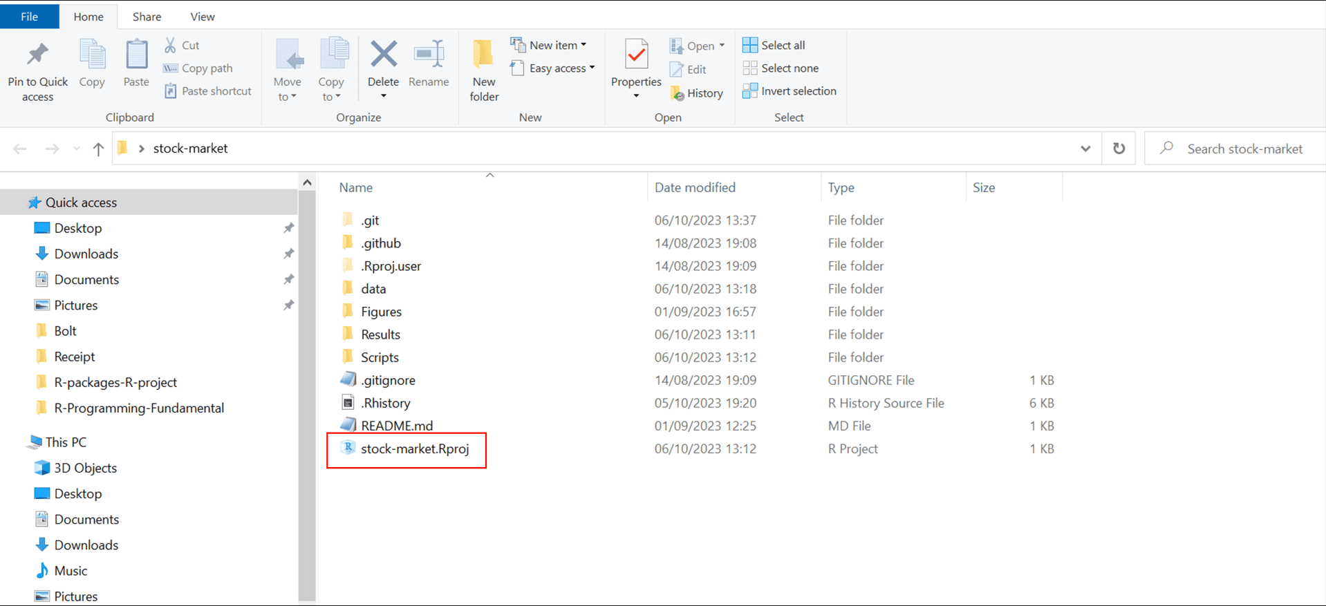
An RStudio Project is an excellent way to keep everything related to your analysis—scripts, data files, figures—all in one organized place. When you set up a project, RStudio automatically sets the working directory to your project folder. This feature is incredibly helpful because it keeps file paths consistent and makes your work reproducible, no matter where it’s opened. For example, here’s a look at how an RStudio project might be organized, as shown in Figure 4.3.

Figure 4.3: Organization of an R Project Directory

4.4.3.1 Creating a New RStudio Project

Let’s create a new RStudio project. You can do this by following these simple steps:

1. Go to: File → New Project

2. Choose: Existing Directory

Figure 4.4: Creating a New Project in RStudio

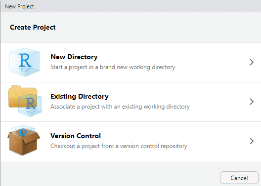
3. Select the folder you want as your project’s working directory.

4. Click: Create Project

Figure 4.5: Creating a New R Project from an Existing Directory

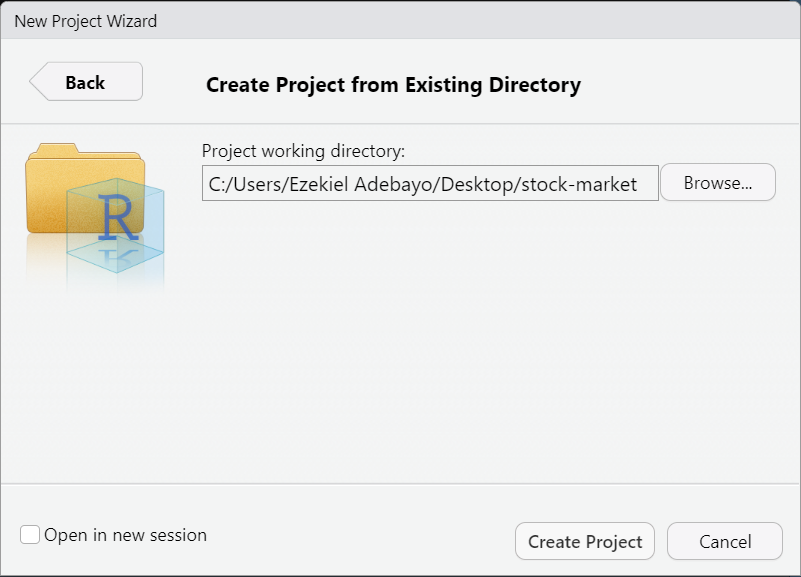
Once you click “Create Project”, you’re all set! You’ll be inside your new RStudio project.

Figure 4.6: RStudio Project: Stock Market Price Scraper Using R

To open this project later, just click the .Rproj file in your project folder, and you’ll be right back in the organized workspace you set up.

Figure 4.7: Organization of an R Project Directory

4.5 Experiment 4.3: Importing and exporting data in R

Data import and export are essential steps in data science. With R, you can bring in data from spreadsheets, databases, and many other formats, then save your processed results. Some of the popular R packages for data import are shown in Figure 4.8:

Figure 4.8: Data Import Packages in R

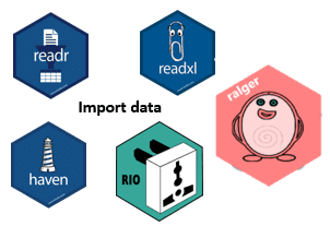
Note

Packages like readr, readxl, and haven are part of the tidyverse, so they come pre-installed with it—no need for separate installations. Here’s a full list of tidyverse packages:

tidyverse::tidyverse_packages()

#>  [1] "broom"         "conflicted"    "cli"           "dbplyr"       
#>  [5] "dplyr"         "dtplyr"        "forcats"       "ggplot2"      
#>  [9] "googledrive"   "googlesheets4" "haven"         "hms"          
#> [13] "httr"          "jsonlite"      "lubridate"     "magrittr"     
#> [17] "modelr"        "pillar"        "purrr"         "ragg"         
#> [21] "readr"         "readxl"        "reprex"        "rlang"        
#> [25] "rstudioapi"    "rvest"         "stringr"       "tibble"       
#> [29] "tidyr"         "xml2"          "tidyverse"

Note

You don’t need to install any of these packages individually since they’re all included with the tidyverse installation.

4.5.1 Packages for Reading and Writing Data in R

R programming has some fantastic packages that make importing and exporting data simple and straightforward. Let’s go through a few of the most commonly used packages and functions that you’ll need to know when working with data in R.

readr Package

The readr package is your go-to for handling CSV files, which are very common in data analysis. Here are the two main functions you’ll use:

• read_csv(): This function lets you import data from a CSV file into R as a data frame. Think of it as loading your data from a spreadsheet directly into R for analysis.

• write_csv(): Once you’re done with your data analysis and want to save your results, this function exports your data frame to a CSV file. It’s great for sharing your data or saving a backup!

readxl Package

The readxl package is specifically designed for Excel files. This is super useful if you’re working with .xlsx files.

• read_xlsx(): Use this function to import an Excel file directly into R. It’s similar to read_csv() but for Excel formats.

writexl Package

When you need to export your data to an Excel file, writexl is a handy package to have.

• write_xlsx(): This function allows you to export your data frame to an Excel file. Perfect for sharing your work with colleagues who prefer Excel!

haven Package

The haven package is here to help when you’re working with data from statistical software like SPSS and Stata.

• read_sav(): This function imports data from SPSS files (files with .sav extension) into R.

• write_sav(): Exports a data frame from R back to SPSS format.

• read_dta(): For Stata users, this function imports Stata files into R.

• write_dta(): Similarly, this function lets you export data frames to Stata format.

rio Package

The rio package is like the Swiss Army knife of data import and export. It can handle multiple file types, so you don’t need to remember specific functions for each format.

• import(): Use this function to import data from nearly any file type—CSV, Excel, SPSS, Stata, you name it.

• export(): Just like import(), this function can export your data frame to a wide variety of formats.

Tip

For more details on all the options available with rio package, check out the rio documentation.

4.5.2 Working with Projects in RStudio

When we’re working on projects in R, especially those that involve reading and writing data, it’s best to set up an RStudio project. An RStudio project automatically manages your working directory, making sure you’re always in the right folder, which is essential when importing and exporting data. By using relative paths (like data/my_file.csv), your code becomes more portable and less dependent on your specific folder structure.

In practice, this setup will save you from having to manually set or adjust your working directory every time you start R. So when you’re working in a project, loading and saving files becomes as easy as referencing their relative file paths.

Example: Importing CSV Data

Let’s practice importing data using the gapminder.csv file.

Instructions:

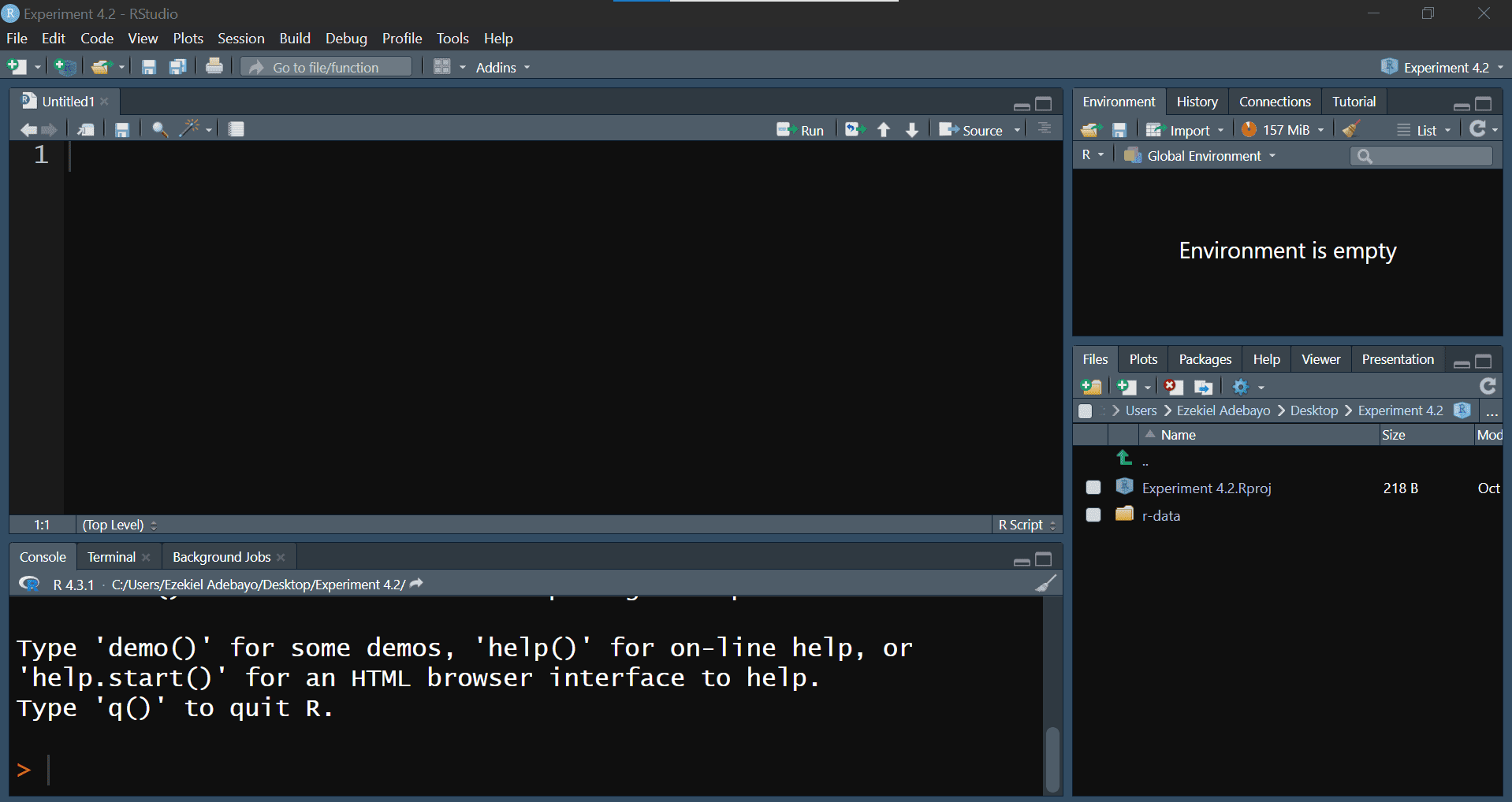
1. Create a Directory: Make a new folder on your desktop called Experiment 4.2.

2. Download Data: Go to to Google Drive to download the r-data folder (see Section A.1 for more information). Once downloaded, unzip the folder and move it into your Experiment 4.2 folder.

3. Create an RStudio Project: Now, open RStudio and set up a new project:

   • Go to File > New Project.

   • Select Existing Directory and browse to your Experiment 4.2 folder.

   • This project setup will organize your work and keep everything related to this experiment in one place.

Your project structure should resemble what’s shown in Figure 4.9:

Figure 4.9: Starting a New R Project in RStudio

Now, let’s import the gapminder.csv file from the r-data folder into R. We’ll use the tidyverse package for easy data manipulation and visualization.

library(tidyverse)
library(readxl) # For reading Excel files
library(haven) # For reading SPSS/Stata/SAS files

# Load the gapminder data

gapminder <- read_csv("r-data/gapminder.csv")

#> Rows: 1704 Columns: 6
#> ── Column specification ────────────────────────────────────────────────────────
#> Delimiter: ","
#> chr (2): country, continent
#> dbl (4): year, lifeExp, pop, gdpPercap
#> 
#> ℹ Use `spec()` to retrieve the full column specification for this data.
#> ℹ Specify the column types or set `show_col_types = FALSE` to quiet this message.

# Exploring the data
names(gapminder)

#> [1] "country"   "continent" "year"      "lifeExp"   "pop"       "gdpPercap"

dim(gapminder)

#> [1] 1704    6

head(gapminder)

summary(gapminder)

#>    country           continent              year         lifeExp     
#>  Length:1704        Length:1704        Min.   :1952   Min.   :23.60  
#>  Class :character   Class :character   1st Qu.:1966   1st Qu.:48.20  
#>  Mode  :character   Mode  :character   Median :1980   Median :60.71  
#>                                        Mean   :1980   Mean   :59.47  
#>                                        3rd Qu.:1993   3rd Qu.:70.85  
#>                                        Max.   :2007   Max.   :82.60  
#>       pop              gdpPercap       
#>  Min.   :6.001e+04   Min.   :   241.2  
#>  1st Qu.:2.794e+06   1st Qu.:  1202.1  
#>  Median :7.024e+06   Median :  3531.8  
#>  Mean   :2.960e+07   Mean   :  7215.3  
#>  3rd Qu.:1.959e+07   3rd Qu.:  9325.5  
#>  Max.   :1.319e+09   Max.   :113523.1

After running this script, you should see your dataset loaded into RStudio, ready for exploration. Your script should look like the one in Figure 4.10:

Figure 4.10: Loading and Exploring Data in RStudio

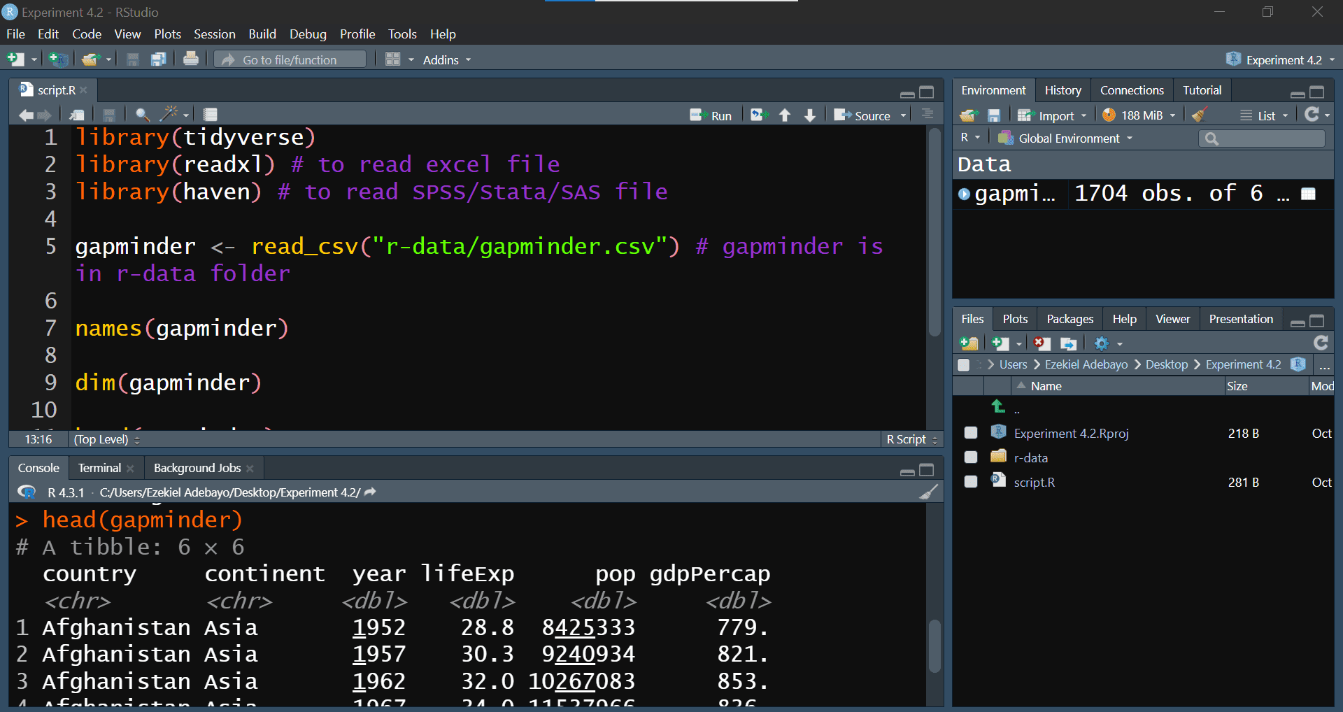
With this setup, you’re ready to dive into analyzing the gapminder data in R! If you’re working with other file formats like Excel or SPSS, check out Section 4.5.1 for detailed instructions on how to import these file types into R.

Example: Exporting Data Frames

Exporting data from R is straightforward. For example, to export the gapminder data frame as an Excel file:

library(writexl)

write_xlsx(gapminder, "gapminder_nigeria.xlsx")

This will create an Excel file in your project directory as shown in Figure 4.11:

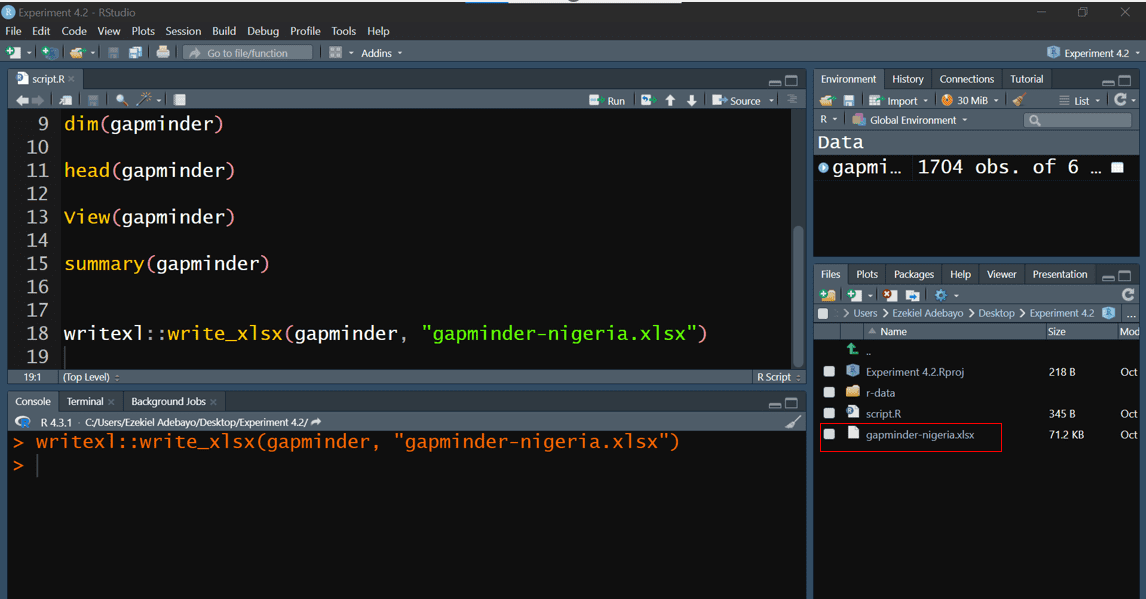
Figure 4.11: Exporting Data to Excel in RStudio using write_xlsx()function

4.6 Experiment 4.4: Dealing with Missing Data in R

Missing data is a common issue in data analysis. Recognizing and handling missing values appropriately is crucial for accurate analyses. R provides several functions to help you deal with missing data.

4.6.1 Recognizing Missing Values

In R, missing values are represented by NA. Identifying these missing values is crucial for accurate data analysis. Here are some functions to check for missing data:

• is.na(): Returns a logical vector indicating which elements are NA.

x <- c(1, 2, NA, 4, NA, 6)

is.na(x)

#> [1] FALSE FALSE  TRUE FALSE  TRUE FALSE

• anyNA(): Checks if there are any NA values in an object. It returns TRUE if there is at least one NA, and FALSE otherwise.

anyNA(x)

#> [1] TRUE

Let’s apply anyNA() function to a sample salary_data data frame:

salary_data <- data.frame(
  Name = c("Alice", "Francisca", "Fatima", "David"),
  Age = c(25, NA, 30, 35),
  Salary = c(50000, 52000, NA, 55000)
)

salary_data

In this data frame, we have missing values for Francisca’s age and Fatima’s salary. We can use anyNA() to check for any missing values:

anyNA(salary_data)

#> [1] TRUE

This indicates that there are missing values in the data frame. You can also check for missing values in specific columns:

anyNA(salary_data$Age)

#> [1] TRUE

And for the Name column:

anyNA(salary_data$Name)

#> [1] FALSE

• complete.cases(): Returns a logical vector indicating which rows (cases) are complete, meaning they have no missing values. For example, using our sample salary_data data frame:

salary_data

complete.cases(salary_data)

#> [1]  TRUE FALSE FALSE  TRUE

This indicates that rows 2 and 3 contain missing values, meaning rows 2 and 3 are not complete.

If you want to check if there are any missing values across all rows (i.e., if any case is incomplete):

anyNA(complete.cases(salary_data))

#> [1] FALSE

4.6.2 Summarizing Missing Data

After identifying that your dataset contains missing values, it’s essential to quantify them to understand the extent of the issue. Summarizing missing data helps you decide how to handle these gaps appropriately. To count the total number of missing values in your entire dataset, you can use the sum() function combined with is.na(). Remember the is.na() function returns a logical vector where each element is TRUE if the corresponding value in the dataset is NA, and FALSE otherwise. Summing this logical vector gives you the total count of missing values because TRUE is treated as 1 and FALSE as 0 in arithmetic operations.

Example:

Suppose you have a sampled airquality dataset:

airquality_data <- tibble::tribble(~Ozone, ~Soar.R, ~Wind, ~Temp, ~Month, ~Day, 41, 190, 7.4, 67, 5, 1, 36, 118, 8, 72, 5, 2, 12, 149, 12.6, 74, 5, 3, 18, 313, 11.5, 62, NA, 4, NA, NA, 14.3, 56, NA, 5, 28, NA, 14.9, 66, NA, 6, 23, 299, 8.6, 65, 5, 7, 19, 99, 13.8, 59, 5, 8, 8, 19, 20.1, 61, 5, 9, NA, 194, 8.6, 69, 5, 10)

To count the total number of missing values in this dataset, you would use:

sum(is.na(airquality_data))

#> [1] 7

There are 7 missing values in the entire data frame.

Missing Values Per Column:

colSums(is.na(airquality_data))

#>  Ozone Soar.R   Wind   Temp  Month    Day 
#>      2      2      0      0      3      0

This output indicates:

• Ozone column has 2 missing values.

• Solar.R column has 2 missing values.

• Wind column has 0 missing values.

• Temp column has 0 missing values.

• Month column has 3 missing values.

• Daycolumn has 0 missing values.

For a column-wise summary, you can also use the inspect_na() function from the inspectdf package. First, install and load the package:

install.packages("inspectdf")

inspectdf::inspect_na(airquality_data)

4.6.3 Handling Missing Values

There are several strategies to handle missing data:

a. Removing Missing Values:

You can remove rows with missing values using na.omit():

cleaned_data <- na.omit(airquality_data)
cleaned_data

b. Imputation:

Alternatively, you can fill in missing values with estimates like the mean, median, or mode.

For the Ozone column:

airquality_data$Ozone[is.na(airquality_data$Ozone)] <- mean(airquality_data$Ozone, na.rm = TRUE)

For the Month column:

airquality_data$Month[is.na(airquality_data$Month)] <- median(airquality_data$Month, na.rm = TRUE)

To see the result of the imputation, we can call out the airquality_data:

airquality_data

c. Using packages:

For more advanced imputation methods, you can use packages like mice or Hmisc. Additionally, the bulkreadr package simplifies the process:

library(bulkreadr)
fill_missing_values(airquality_data, selected_variables = c("Ozone", "Soar.R"), method = "mean")

You can also use fill_missing_values() to impute all the missing values in the data frame:

fill_missing_values(airquality_data, method = "median")

4.6.4 Exercise 4.1: Medical Insurance Data

In this exercise, you’ll explore the Medical_insurance_dataset.xlsx file located in the r-data folder. You can download this file from Google Drive. This dataset contains medical insurance information for various individuals. Below is an overview of each column:

1. User ID: A unique identifier for each individual.

2. Gender: The individual’s gender (‘Male’ or ‘Female’).

3. Age: The age of the individual in years.

4. AgeGroup: The age bracket the individual falls into.

5. Estimated Salary: An estimate of the individual’s yearly salary.

6. Purchased: Indicates whether the individual has purchased medical insurance (1 for Yes, 0 for No).

Your Tasks:

1. Importing and Basic Handling:

   • Create a new script and import the data from the Excel file.
   • How would you import this data if it’s in SPSS format?
   • Use the clean_names() function from the janitor package to make variable names consistent and easy to work with.
   • Can you display the first three rows of the dataset?
   • How many rows and columns does the dataset have?

2. Understanding the Data:

   • What are the column names in the dataset?
   • Can you identify the data types of each column?
   • How would you handle missing values if there are any?

3. Basic Descriptive Statistics:

   • What is the average age of the individuals in the dataset?
   • What’s the range of the estimated salaries?

4.7 Summary

In Lab 4, you have acquired essential skills to enhance your efficiency and effectiveness as an R programmer:

• Installing and Loading Packages: You learned how to find, install, and load packages from CRAN and external repositories like GitHub.

• Handling and Imputing Missing Data: You explored methods to identify missing values using functions like is.na(), anyNA(), and complete.cases().

• Reproducible Workflows with RStudio Projects: You discovered the importance of organizing your work within RStudio Projects.

• Importing and Exporting Data: You practiced importing and exporting data in various formats (CSV, Excel, SPSS) using packages like readr, readxl, and haven.

These foundational skills are crucial for efficient data analysis in R, enabling you to work with diverse data sources, maintain analysis integrity, and collaborate effectively. Congratulations on advancing your R programming proficiency!

---

1. It is common for a package to print out messages when you load it. These messages often include information about the package version, attached packages, or important notes from the authors. For example, when you load the tidyverse package. If you prefer to suppress these messages, you can use the suppressMessages() function: suppressMessages(library(tidyverse))