3 Writing Custom Functions

In this Lab 3, we will explore how to write your own functions in R. Functions are essential in programming because they allow you to encapsulate code that performs specific tasks. This makes your programs more modular, readable, and easier to maintain. By designing custom functions, you can automate repetitive tasks, streamline your data analysis processes, and enhance the efficiency of your code.

By the end of this lab, you will be able to:

Understand the Syntax of Functions in R
Learn how to define functions using the function() keyword, specify arguments, and structure the function body to perform desired operations.
Create Custom Functions
Write your own functions to perform specific data analysis tasks, allowing you to reuse code and avoid repetition.
Utilize Functions to Modularize and Streamline Code
Break down complex data analysis tasks into smaller, manageable functions to make your code more organized and maintainable.
Understand Variable Scope Within Functions
Grasp how variable scope works in R, distinguishing between local and global variables, and understand how this affects the behavior of your functions.
Apply Best Practices in Function Design
Implement best practices such as choosing meaningful function names, including documentation with comments, handling inputs and outputs effectively, and incorporating error handling.
Demonstrate Understanding Through Practical Application
Use the functions you create in real data analysis scenarios to show how they can simplify tasks and improve code efficiency.

By completing Lab 3, you’ll enhance your programming skills in R, enabling you to write code that is not only effective but also clean, reusable, and easy to understand. These skills are fundamental for any data analysis or data science work you’ll undertake in the future.

3.1 Introduction

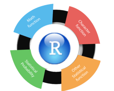
Imagine you want to perform a task repeatedly, like squaring numbers or checking for missing values in a dataset. Instead of writing the same code again and again, you create a function—a reusable block of code that does this task for you! R already has many built-in functions such as such as c(), mean(), print(), class(), length(), but we can also write our own to perform tasks tailored to our needs.

Functions usually take in some form of data structure—like a value, vector, or dataframe—as an argument, process it, and return a result.

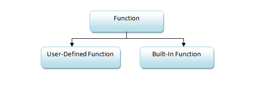
Figure 3.1: Core Functions in R Programming

3.1.1 Types of Functions

Function extends the functionality of R. Broadly, we can categorize functions into two types:

A simple diagram depicting two types of functions in R: User-Defined Functions and Built-In Functions. The diagram shows that all functions in R fall into these two categories, with user-defined functions created by users and built-in functions provided by R for various operations. — Figure 3.2: Types of Functions in R Programming

Built-in Functions: These are pre-defined in R, such as print() and mean().
User-defined Functions: These are functions you create to perform specific tasks.

3.1.2 Why Write Your Own Function?

Creating your own functions has several advantages:

Code Reusability: Functions promote code reuse and help you avoid repetition.
Improved Readability: They make your code more readable and maintainable.
Modular Programming: Functions allow for modular programming, where you can break down complex tasks into smaller, manageable pieces.

3.1.3 When Should You Write a Function?

Consider writing a function whenever you find yourself copying and pasting a block of code more than twice. If you’re repeating the same code, it’s a good indication that a function could simplify your work.

3.2 Experiment 3.1: Creating a Function

There are three key steps to creating a new function:

Function Name: Decide on a descriptive name for your function, such as square_it.
Function Arguments: Specify the inputs your function will accept inside the function() keyword, for example, function(x, y).
Function Body: Write the R code that uses those arguments, enclosed within curly braces {}. This is where you’ll define what the function does with the inputs—whether it’s creating a plot, calculating a statistic, running a regression analysis, etc.

The general structure of a function is as follows:

function_name <- function(argument1, argument2, ...) {
  # Function body
  return(value)
}

Note

Note that the arguments can be any type of object—such as a scalar, matrix, dataframe, vector, or logical—and you don’t need to define what they are beforehand.

If you create an object inside a function that you want to use outside of it, you need to return it using the return() function.

3.2.1 Calling a User-defined Function in R

You can call a user-defined function just like any built-in function, using its name. If the function accepts parameters or arguments, you pass them when calling the function.

3.2.2 Creating a Function to Square a Number

Let’s start by creating a simple function to square a number. This example will introduce you to defining and using functions in R.

Defining the Function:

First, we’ll define the function square_it. This function will take a single input, x, and return its square. Here’s how you would write it:

square_it <- function(x) {
  return(x^2)
}

Now, whenever you call square_it() with a numerical input, it will output the square of that number.

Testing the Function

To verify that the function works as expected, try squaring a few numbers:

Testing with 12:

square_it(12)

#> [1] 144

Testing with 6:

square_it(x = 6)

#> [1] 36

This basic function highlights the usefulness of custom functions in R, enabling specific operations with minimal code.

3.2.3 Checking for Missing Values

Next, let’s create a function that checks for missing values in a dataset and counts them.

Defining the Function

We’ll define a function called check_NA as follows:

check_NA <- function(data) {
  any_na <- anyNA(data)
  na_count <- sum(is.na(data))
  announcement <- paste("Any NA:", any_na, ", Total NA:", na_count)
  return(announcement)
}

Testing the Function

You can use this function to check for missing values in various datasets.

For the airquality dataset:

check_NA(airquality)

#> [1] "Any NA: TRUE , Total NA: 44"

For the iris dataset:

check_NA(iris)

#> [1] "Any NA: FALSE , Total NA: 0"

Running these commands will let you know if there are any missing values in the dataset and provide the total count of missing values.

3.2.4 Data Frame Manipulation Using `switch()`

Suppose we have a data frame containing information about employees. We want to perform different operations on this data frame based on user input. The available operations are:

“summary”: Get a summary of the data frame.
“add_column”: Add a new column to the data frame.
“filter”: Filter the data frame based on a specified condition.
“group_stats”: Calculate group-wise statistics.

To follow along with this example, please refer to Section 1.4.4 for a detailed tutorial and comprehensive understanding of the switch() function.

Step 1: Create a Sample Data Frame

library(tidyverse)

# Sample data frame
staff_data <- data.frame(
  EmployeeID = 1:6,
  Name = c("Alice", "Ebunlomo", "Festus", "TY Bello", "Fareedah", "Testimony"),
  Department = c("HR", "IT", "Finance", "Data Science", "Marketing", "Finance"),
  Salary = c(70000, 80000, 75000, 82000, 73000, 78000)
)

staff_data

Step 2: Define the Function

# Define the function
data_frame_operation <- function(data, operation = "filter" # or any of "summary", "add_column", "filter", "group_stats"
) {
  result <- switch(operation,

    # Case 1: Summary of the data frame
    summary = {
      print("Summary of Data Frame:")
      summary(data)
    },

    # Case 2: Add a new column 'Bonus' which is 10% of the Salary
    add_column = {
      data$Bonus <- data$Salary * 0.10
      print("Data Frame after adding 'Bonus' column:")
      data
    },

    # Case 3: Filter employees with Salary > 75,000
    filter = {
      filtered_data <- filter(data, Salary > 75000)
      print("Filtered Data Frame (Salary > 75,000):")
      filtered_data
    },

    # Case 4: Group-wise average salary
    group_stats = {
      group_summary <- data %>%
        group_by(Department) %>%
        summarize(Average_Salary = mean(Salary))
      print("Group-wise Average Salary:")
      group_summary
    },

    # Default case
    {
      print("Invalid operation. Please choose a valid option.")
      NULL
    }
  )

  # Return the result
  return(result)
}

Explanation:

Function data_frame_operation:
- Parameters:
  - data: The data frame to operate on.
  - operation: A string specifying the operation to perform.
- Using switch():
  - Each case corresponds to a specific operation.
  - Cases that involve multiple expressions are wrapped in {}.
  - The last expression in the block is returned as the result of the case.
  - If no match is found, the final unnamed argument serves as the default case.
- Operations:
  - “summary”: Provides a summary of the data frame.
  - “add_column”: Adds a new column Bonus (10% of Salary) to the data frame.
  - “filter”: Filters the data frame to include only employees with a salary greater than $75,000.
  - “group_stats”: Calculates the average salary for each department.
- Default Case: Prints an error message and returns NULL if the operation is invalid.
- Return Value: The result of the operation is returned by the function.

Step 3: Use the Function

Let’s test the function with different operations.

Example 1: Summary of the Data Frame

# Perform the 'summary' operation
data_frame_operation(staff_data, "summary")

#> [1] "Summary of Data Frame:"

#>    EmployeeID       Name            Department            Salary     
#>  Min.   :1.00   Length:6           Length:6           Min.   :70000  
#>  1st Qu.:2.25   Class :character   Class :character   1st Qu.:73500  
#>  Median :3.50   Mode  :character   Mode  :character   Median :76500  
#>  Mean   :3.50                                         Mean   :76333  
#>  3rd Qu.:4.75                                         3rd Qu.:79500  
#>  Max.   :6.00                                         Max.   :82000

Example 2: Add a New Column

# Perform the 'add_column' operation
data_frame_operation(staff_data, "add_column")

#> [1] "Data Frame after adding 'Bonus' column:"

Example 3: Filter the Data Frame

# Perform the 'filter' operation
data_frame_operation(staff_data, "filter")

#> [1] "Filtered Data Frame (Salary > 75,000):"

Example 4: Group-wise Statistics

# Perform the 'group_stats' operation
data_frame_operation(staff_data, "group_stats")

#> [1] "Group-wise Average Salary:"

Example 5: Invalid Operation

# Attempt an invalid operation
data_frame_operation(staff_data, "view")

#> [1] "Invalid operation. Please choose a valid option."

#> NULL

3.2.5 Exercise 3.1.1: Temperature Conversion

Now, it’s your turn to create a function.

Your Task: Create a function to convert Celsius (C) to Fahrenheit (F). You can use the formula:

$\text{F} = \text{C} \times 1.8 + 32$

Instructions:

Define the Function
- Name the function celsius_to_fahrenheit.
- It should take one argument, the temperature in Celsius.
Implement the Formula
- Inside the function, apply the formula to convert Celsius to Fahrenheit.
Return the Result
- The function should return the Fahrenheit temperature.

Test Your Function:

Use your function to convert the following Celsius temperatures to Fahrenheit:

100°C
75°C
120°C

For each temperature, call your function and verify that it returns the correct Fahrenheit value.

3.2.6 Exercise 3.1.2: Pythagoras Theorem

Create a function to :

Your Task: Create a function called pythagoras to calculate the hypotenuse (c) of a right-angled triangle using Pythagoras’ theorem:

\[c = \sqrt{a^2 + b^2}\]

where a and b are the lengths of the other two sides.

A geometric diagram of a triangle, showing three connected lines forming a triangle shape. — Figure 3.3: Geometric Representation: Right-Angled Triangle

Instructions:

Define the Function
- Name the function pythagoras.
- It should take two arguments: a and b.
Implement the Formula
- Inside the function, calculate the hypotenuse using the Pythagorean theorem.
Return the Result
- The function should return the length of the hypotenuse.

Test Your Function:

Use your pythagoras function to calculate the hypotenuse for the following triangles:

For $a = 4.1$ and $b = 2.6$
For $a = 3$ and $b = 4$

Call your function with these values and verify that it returns the correct hypotenuse length.

3.2.7 Exercise 3.1.3: Staff Data Manipulation Using `switch()`

Based on the example in Section 3.2.4, try modifying the code to include an additional operation:

“raise_salary”: Increase the salary of all employees by 5%.

Instructions:

Add a new case to the switch() function for "raise_salary".
In this case, increase the Salary column by 5% and return the updated data frame.
Test the code by setting operation = "raise_salary".

Your Task:

# Modify the function to include 'raise_salary' operation
data_frame_operation <- function(..., operation) {
  result <- switch(operation,

    # Existing cases...

    # Case for 'raise_salary'
    raise_salary = {
      data$Salary <- data$Salary * ...
      print("Data Frame after 5% salary increase:")
      data
    },

    # Default case
    {
      print("Invalid operation. Please choose a valid option.")
      NULL
    }
  )

  # Return the result
  return(...)
}

Test the New Operation

# Perform the 'raise_salary' operation
data_frame_operation(staff_data, "---")

Replace the ... with the correct values and complete the exercise!

3.3 Experiment 3.2: Understanding Variable Scope Within Functions

When writing functions in R, it’s crucial to understand how variables behave inside and outside those functions. This concept is known as variable scope. Variable scope determines where a variable is accessible in your code and how changes to variables within functions can affect variables outside of them.

3.3.1 Local vs. Global Variables

Local Variables: These are variables that are defined within a function. They exist only during the execution of that function and are not accessible outside of it.
Global Variables: These are variables that are defined outside of any function. They exist in the global environment and can be accessed by any part of your script, including inside functions (unless shadowed by a local variable of the same name).

3.3.2 How Variable Scope Works in R

In R, each function has its own environment. This means that variables created inside a function (local variables) do not interfere with variables outside the function (global variables), even if they have the same name.

Example: Local Variable

Let’s look at an example to illustrate this:

greet <- function() {
  announcement <- "Hello from inside the function!"
  print(announcement)
}

greet() # This will print the announcement defined inside the function

#> [1] "Hello from inside the function!"

print(announcement) # This will result in an error because 'announcement' is not defined globally

#> Error: object 'announcement' not found

In this example, announcement is a local variable within the greet function. Trying to access announcement outside the function results in an error because it doesn’t exist in the global environment.

Example: Global Variable Access

Functions in R can access global variables unless there is a local variable with the same name:

announcement <- "Hello from the global environment!"

greet <- function() {
  print(announcement)
}

greet() # This will print "Hello from the global environment!"

#> [1] "Hello from the global environment!"

Here, the function greet accesses the global variable announcement because there is no local variable named announcement inside the function.

3.3.3 Variable Shadowing

If a local variable inside a function has the same name as a global variable, the local variable will shadow the global one within that function:

announcement <- "Hello from the global environment!"

greet <- function() {
  announcement <- "Hello from inside the function!"
  print(announcement)
}

greet() # Prints: Hello from inside the function!

#> [1] "Hello from inside the function!"

print(announcement) # Prints: Hello from the global environment!

#> [1] "Hello from the global environment!"

In this case, the announcement variable inside greet is local and doesn’t affect the global announcement variable.

3.4 Summary

In this lab, you have developed essential skills in creating custom functions in R:

Understanding the syntax of functions in R, including how to define functions using the function() keyword, specify arguments, and structure the function body.
Creating and utilizing your own custom functions to perform specific data analysis tasks, promoting code reuse and avoiding repetition.
Applying functions to modularize and streamline your code, breaking down complex tasks into smaller, manageable pieces for better organization and maintainability.
Grasping variable scope within functions, distinguishing between local and global variables, and understanding how this affects the behavior of your functions.
Implementing best practices in function design, such as choosing meaningful function names, including documentation with comments, handling inputs and outputs effectively, and incorporating error handling.

These skills are fundamental for efficient programming in R and will greatly enhance your data analysis capabilities. They form a strong foundation for more advanced topics you will encounter as you continue learning. Congratulations on advancing your programming expertise!

In the next lab, we’ll delve into managing packages, creating reproducible workflows using RStudio project, and reading data from a file.

3.1 Introduction

3.1.1 Types of Functions

3.1.2 Why Write Your Own Function?

3.1.3 When Should You Write a Function?

3.2 Experiment 3.1: Creating a Function

3.2.1 Calling a User-defined Function in R

3.2.2 Creating a Function to Square a Number

3.2.3 Checking for Missing Values

3.2.4 Data Frame Manipulation Using switch()

Step 1: Create a Sample Data Frame

Step 2: Define the Function

Step 3: Use the Function

Example 1: Summary of the Data Frame

Example 2: Add a New Column

Example 3: Filter the Data Frame

Example 4: Group-wise Statistics

Example 5: Invalid Operation

3.2.5 Exercise 3.1.1: Temperature Conversion

3.2.6 Exercise 3.1.2: Pythagoras Theorem

3.2.7 Exercise 3.1.3: Staff Data Manipulation Using switch()

Test the New Operation

3.3 Experiment 3.2: Understanding Variable Scope Within Functions

3.3.1 Local vs. Global Variables

3.3.2 How Variable Scope Works in R

Example: Local Variable

Example: Global Variable Access

3.3.3 Variable Shadowing

3.4 Summary

3.2.4 Data Frame Manipulation Using `switch()`

3.2.7 Exercise 3.1.3: Staff Data Manipulation Using `switch()`