2 Understanding Data Structures
In this Lab 2, we’ll explore the fundamental data structures that are essential for data analysis in R: vectors, matrices, data frames, and lists. Mastering these structures will enable you to handle data efficiently and perform various operations crucial for statistical analysis and data science tasks.
By the end of this lab, you will be able to:
Identify Fundamental Data Structures
Recognize and describe the key characteristics of vectors, matrices, data frames, and lists in R.Create Data Structures
Construct vectors, matrices, data frames, and lists using appropriate functions and syntax in R.Manipulate Data Structures
Perform operations such as indexing, slicing, and modifying elements within vectors, matrices, data frames, and lists.Apply Appropriate Operations and Functions
Utilize relevant R functions and operators to perform calculations and transformations specific to each data type.Demonstrate Understanding Through Application
Solve problems and complete exercises that require the correct application of operations and functions to manipulate and analyze data within these structures.
By completing Lab 2, you’ll build a solid foundation in handling data structures in R, which is crucial for more advanced data analysis and programming tasks.
2.1 Introduction
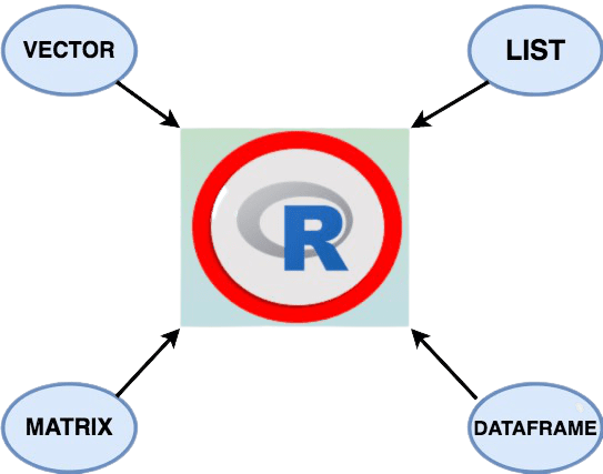
R offers several fundamental data structures to handle diverse data and analytical needs. These include vectors, matrices, factors, data frames, and lists.
2.2 Experiment 2.1: Vectors
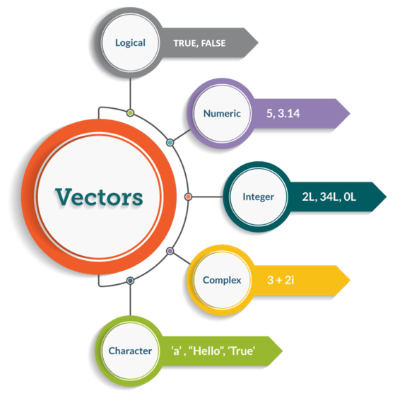
A vector is a one-dimensional array that holds elements of the same data type. This is the most basic and frequently used data structure in R.
2.2.1 Creating a Vector
To create a vector, use the c() function:
gender <- c("Male", "Female", "Female", "Male", "Female", "Male")Adding a space after every comma in c() makes your code more readable:
covid_confirmed <- c(31, 30, 37, 25, 33, 34, 26, 32, 23, 45)

covid_confirmed
#> [1] 31 30 37 25 33 34 26 32 23 45You can check the class of the vector using the class() function:
class(covid_confirmed)#> [1] "numeric"2.2.2 Factor vectors
A categorical variable where each level is a category will be of type factor. For example, gender is a categorical variable with two levels: “Male” or “Female”.
You can create a factor vector directly using the factor() function:
#> [1] Male   Female Female Male   Female
#> Levels: Female Male
Check the class and levels:
class(gender_factor) # Returns "factor"#> [1] "factor"levels(gender_factor) # Returns "Female" "Male"#> [1] "Female" "Male"If you already have a character vector, convert it to a factor vector using as.factor():
gender <- c("Male", "Female", "Female", "Male", "Female")

gender_factor <- as.factor(gender)

gender_factor
#> [1] Male Female Female Male Female
#> Levels: Female Maleclass(gender_factor)#> [1] "factor"levels(gender_factor)#> [1] "Female" "Male"2.2.3 Length of a vector
Find the length of a vector using the length() function:
2.2.4 Arithmetic Operations with Vectors
Operations with vector are performed element-wise.
2.2.5 Vector selection
To select elements of a vector, use square brackets [ ] and indicate the index of elements to select. R indexing starts at 1.
For example:
| Weekday | Monday | Tuesday | Wednesday | Thursday | Friday | Saturday | Sunday |
|---|---|---|---|---|---|---|---|
| index | 1 | 2 | 3 | 4 | 5 | 6 | 7 |
weekday <- c("Monday", "Tuesday", "Wednessday", "Thursday", "Friday", "Saturday", "Sunday")Access the first element:
weekday[1]#> [1] "Monday"Access the second element:
weekday[2]#> [1] "Tuesday"2.2.6 Exercise 2.1.1: Vector Selection
Given the quiz scores of 13 students:
10, 15, 10, 9, 18, 16, 14, 12, 16, 13, 15, 20, 17.
Create a vector named
scorecontaining the data.Access individual scores of the 1st, 5th, and 10th students.
Access them all together.
2.3 Experiment 2.2: Matrices
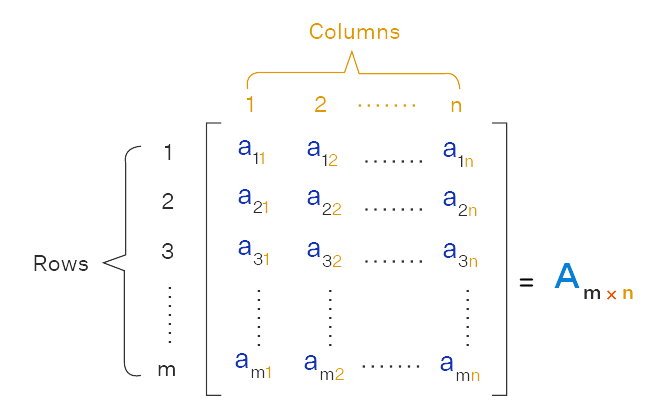
A matrix is a two-dimensional data structure consisting of a rectangular array of elements of the same data type, organized into rows and columns. Figure 2.3 illustrates how matrices are typically represented in mathematics.
2.3.1 Creating Matrices
To create a matrix, use the matrix() function:
matrix(data, nrow, ncol, byrow = FALSE)where:
data: Elements to arrange in the matrix.nrow: Number of rows.ncol: Number of columns.byrow: Fill matrix by rows ifTRUE.
Create the matrix A:
\[A = \begin{pmatrix} 1&-2& 5\\ -3&9&4\\ 5&0&6 \end{pmatrix}\]
#>      [,1] [,2] [,3]
#> [1,]    1   -2    5
#> [2,]   -3    9    4
#> [3,]    5    0    6
Create the matrix B:
\[B = \begin{pmatrix} 2&-8& 14\\ 4&10&16\\ 6&12&18 \end{pmatrix}\]
2.3.2 Matrices slicing
Accessing elements in a matrix is done by using [row, column], between the square brackets, you indicate the position of the row and column in which the elements to access are. For example, to access the element in the first row and second column of matrix A, you type A[1, 2]. To access the element in the third row and second column of matrix A, you type A[3, 2].
A[1, 2] # Element in first row, second column#> [1] -2A[3, 2] # Element in third row, second column#> [1] 02.3.3 Arithmetic Operation in Matrices
You can perform arithmetic operations on matrices. Consider the following matrices
\[A = \begin{pmatrix} 1&-2& 5\\ -3&9&4\\ 5&0&6 \end{pmatrix}\]
\[B = \begin{pmatrix} 2&-8& 14\\ 4&10&16\\ 6&12&18 \end{pmatrix}\]
Addition
A + B#> [,1] [,2] [,3]
#> [1,] 3 6 19
#> [2,] 1 19 20
#> [3,] 11 12 24Multiplication
Matrix multiplication is done using %*% operator:
A %*% B#> [,1] [,2] [,3]
#> [1,] 24 48 72
#> [2,] 54 114 174
#> [3,] 46 112 1782.3.4 Exercise 2.2.1: Matrix Transpose
Consider the following matrix \(A\):
\[A = \begin{pmatrix} 1 & 3 & 5 \\ 2 & 4 & 6 \end{pmatrix}\]
Your Task:
Find the transpose of matrix \(A\), denoted as \(A^{T}\).
Tip
Define matrix \(A\), then use t(A) to find its transpose.
Here’s a starting point for your code:
Replace the ... with the correct values and complete the exercise!
2.3.5 Exercise 2.2.2: Matrix Inverse Multiplication
Given the matrices \(A\) and \(B\) below:
\[A = \begin{pmatrix} 4 & 7 \\ 2 & 6 \end{pmatrix}\]
\[ B = \begin{pmatrix} 3 & 5 \\ 1 & 2 \end{pmatrix}\]
Your Task:
Calculate \(A^{-1} \times B\), where \(A^{-1}\) is the inverse of matrix \(A\).
Hint:
Use the
solve()function in R to find the inverse of matrix \(A\).Use the matrix multiplication operator
%*%to multiply \(A^{-1}\) by \(B\).
Here’s a starting point for your code:
Replace the ... with the correct values for your matrices and complete the exercise!
2.4 Experiment 2.3: Data frame
A data frame is a versatile table-like structure, allowing columns of different data types. It has variables as columns and observations as rows, similar to a spreadsheet or a SQL table.
2.4.1 Creating a Data Frame
To create a data frame, use the data.frame() function:
demographic_data <- data.frame(
  age = c(16, 18, 13, 17, 22),
  gender = c("Female", "Female", "Male", "Female", "Male"),
  bank_account = c(TRUE, FALSE, FALSE, TRUE, FALSE)
)

demographic_data
The number 1 2 3 4 5 at the left hand side on your console are row labels. Also, each column in a data frame is a vector.
Example: COVID 19 Data Frame
Create a data frame with columns states, confirmed cases, recovered cases and death cases.
states <- c("Lagos", "FCT", "Plateau", "Kaduna", "Rivers", "Oyo")

confirmed_cases <- c(58033, 19753, 9030, 8998, 7018, 6838)

recovered_cases <- c(56990, 19084, 8967, 8905, 6875, 6506)

death_cases <- c(439, 165, 57, 65, 101, 123)

covid_19 <- data.frame(states, confirmed_cases, recovered_cases, death_cases)

covid_19
2.4.2 Exploring Data Frames
When working with large datasets, it’s useful to show only part of the data.
1. head(): Shows the first observations.
2. tail(): Shows the last observations.
Both head() and tail() print a top line called header, which contains the names of the different variables in your data set.
Another method that is often used to get a rapid overview of your dataset is the function str().
3. str(): shows you the structure of your dataset. The structure of a data frame tells you:
- The total number of observations
- The total number of variables
- A full list of the variables names
- The first observations
Applying the str() function will often be the first thing that you do when receiving a new dataset. It is a great way to get more insight in your dataset before diving into the real analysis.
4. names(): Prints each column name.
5. nrow(): Returns the number of rows.
6. ncol(): Returns the number of columns.
7. dim(): Returns the number of rows and columns.
8. View(): Opens a spreadsheet-style data viewer (in RStudio).
9. summary(): Returns summary statistics of all columns.
Consider the following vectors:
Create a data frame:
medical_data <- data.frame(gender, height, weight, bmi)2.4.3 Explore the data
First six observations:
head(medical_data)Last six observations:
tail(medical_data) # To get the last 6 observationColumn names:
names(medical_data)#> [1] "gender" "height" "weight" "bmi"You can also use:
colnames(medical_data)#> [1] "gender" "height" "weight" "bmi"View the dataset (in RStudio):
View(medical_data)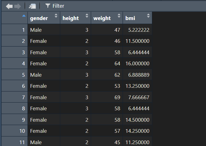
Descriptive statistics:
summary(medical_data)#> gender height weight bmi
#> Length:120 Min. :1.000 Min. :37.00 Min. : 2.375
#> Class :character 1st Qu.:2.000 1st Qu.:50.00 1st Qu.: 6.333
#> Mode :character Median :2.000 Median :56.00 Median :11.000
#> Mean :2.433 Mean :55.58 Mean :12.384
#> 3rd Qu.:3.000 3rd Qu.:62.00 3rd Qu.:14.312
#> Max. :4.000 Max. :78.00 Max. :63.0002.4.4 Built-in Datasets
There are several ways to find the included datasets in R. Using data() will give you a list of available dataset.
data()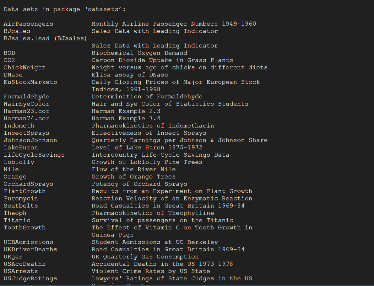
For example, to load the built-in dataset iris, use:
and to load the built-in dataset airquality, use:
To get help on a built-in dataset, such as airquality, use:
?airquality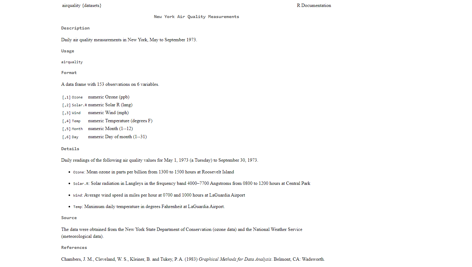
2.4.5 Subsetting Data Frames
Every column in a data frame has a name and if you can recall, we can print the names attribute of a data frame, iris, by using:
names(iris)#> [1] "Sepal.Length" "Sepal.Width" "Petal.Length" "Petal.Width"
#> [5] "Species"and to access a specific column in a data frame by name, you will use the $ operator in the form of df$colname, where df is the name of the data frame and colname is the name of the column you are interested in. This operation will then return the column you want as a vector.
Access specific columns using the $ operator
Use the $ operator to get a vector of Sepal.Length from the iris data frame:
iris$Sepal.Length#> [1] 5.1 4.9 4.7 4.6 5.0 5.4 4.6 5.0 4.4 4.9 5.4 4.8 4.8 4.3 5.8 5.7 5.4 5.1
#> [19] 5.7 5.1 5.4 5.1 4.6 5.1 4.8 5.0 5.0 5.2 5.2 4.7 4.8 5.4 5.2 5.5 4.9 5.0
#> [37] 5.5 4.9 4.4 5.1 5.0 4.5 4.4 5.0 5.1 4.8 5.1 4.6 5.3 5.0 7.0 6.4 6.9 5.5
#> [55] 6.5 5.7 6.3 4.9 6.6 5.2 5.0 5.9 6.0 6.1 5.6 6.7 5.6 5.8 6.2 5.6 5.9 6.1
#> [73] 6.3 6.1 6.4 6.6 6.8 6.7 6.0 5.7 5.5 5.5 5.8 6.0 5.4 6.0 6.7 6.3 5.6 5.5
#> [91] 5.5 6.1 5.8 5.0 5.6 5.7 5.7 6.2 5.1 5.7 6.3 5.8 7.1 6.3 6.5 7.6 4.9 7.3
#> [109] 6.7 7.2 6.5 6.4 6.8 5.7 5.8 6.4 6.5 7.7 7.7 6.0 6.9 5.6 7.7 6.3 6.7 7.2
#> [127] 6.2 6.1 6.4 7.2 7.4 7.9 6.4 6.3 6.1 7.7 6.3 6.4 6.0 6.9 6.7 6.9 5.8 6.8
#> [145] 6.7 6.7 6.3 6.5 6.2 5.9Use the $ operator to get a vector of Species from the iris data frame:
iris$Species#> [1] setosa setosa setosa setosa setosa setosa
#> [7] setosa setosa setosa setosa setosa setosa
#> [13] setosa setosa setosa setosa setosa setosa
#> [19] setosa setosa setosa setosa setosa setosa
#> [25] setosa setosa setosa setosa setosa setosa
#> [31] setosa setosa setosa setosa setosa setosa
#> [37] setosa setosa setosa setosa setosa setosa
#> [43] setosa setosa setosa setosa setosa setosa
#> [49] setosa setosa versicolor versicolor versicolor versicolor
#> [55] versicolor versicolor versicolor versicolor versicolor versicolor
#> [61] versicolor versicolor versicolor versicolor versicolor versicolor
#> [67] versicolor versicolor versicolor versicolor versicolor versicolor
#> [73] versicolor versicolor versicolor versicolor versicolor versicolor
#> [79] versicolor versicolor versicolor versicolor versicolor versicolor
#> [85] versicolor versicolor versicolor versicolor versicolor versicolor
#> [91] versicolor versicolor versicolor versicolor versicolor versicolor
#> [97] versicolor versicolor versicolor versicolor virginica virginica
#> [103] virginica virginica virginica virginica virginica virginica
#> [109] virginica virginica virginica virginica virginica virginica
#> [115] virginica virginica virginica virginica virginica virginica
#> [121] virginica virginica virginica virginica virginica virginica
#> [127] virginica virginica virginica virginica virginica virginica
#> [133] virginica virginica virginica virginica virginica virginica
#> [139] virginica virginica virginica virginica virginica virginica
#> [145] virginica virginica virginica virginica virginica virginica
#> Levels: setosa versicolor virginicaBecause the $ operator returns a vector, you can easily calculate descriptive statistics on columns of a data frame by applying your favorite vector function (like mean(), sd(), or table()) to a column using $.
Let’s calculate the mean of Sepal.Length with themean() function and the frequency of each Species with the table()function in the iris data frame:
mean(iris$Sepal.Length)#> [1] 5.843333table(iris$Species)#>
#> setosa versicolor virginica
#> 50 50 50Access elements using [row, column]
Just like a matrix, you can access specific data in a data frame by using [row, column], where rows and columns are vectors of integers.
| Data Frame Slicing | Interpretation |
|---|---|
data[1, ] |
First row and all columns |
data[, 2] |
All rows and second column |
data[c(1, 3, 5), 2] |
Rows 1, 3, 5 and column 2 only |
data[1:3, c(1, 3)] |
First three rows and columns 1 and 3 only |
data or data[, ]
|
All rows and all columns |
| Data Frame Slicing in R | |
|---|---|
| Examples and Interpretations | |
| Data Frame Slicing | Interpretation |
| data[1, ] | First row and all columns |
| data[, 2] | All rows and second column |
| data[c(1, 3, 5), 2] | Rows 1, 3, 5 and column 2 only |
| data[1:3, c(1, 3)] | First three rows and columns 1 and 3 only |
| data or data[, ] | All rows and all columns |
2.4.6 Exercise 2.3.1: Subsetting a Dataframe
Using the airquality dataset:
Examine the
airqualitydataset.Select the first three columns.
Select rows
1-3and columns1and3.Select rows
1-5and column1.Select the first row.
Select the first 6 rows .
2.5 Experiment 2.4: Lists
A list in R is like a container that can hold various elements, such as vectors, matrices, data frames, and even other lists.
2.5.1 Creating a List
Use the list() function to create a list:
my_list <- list(
  age = 19,
  gender = "Male",
  pass = TRUE
)
Here, my_list consists of three components:
age: Numeric value.gender: Character string.pass: Logical value.
2.5.2 Accessing List Elements
To show the contents of a list you can simply type its name as any other object in R:
my_list#> $age
#> [1] 19
#>
#> $gender
#> [1] "Male"
#>
#> $pass
#> [1] TRUEYou can extract individual element in a list by using double square brackets [[ ]]. For example,
my_list[[1]] # Returns 19#> [1] 19my_list[["age"]] # Returns 19#> [1] 19Using single square brackets [ ] returns a list containing the element.
my_list[1]#> $age
#> [1] 192.6 Summary
In this lab 2, you have acquired foundational skills in R’s basic data structures:
Understanding the characteristics and differences between vectors, matrices, data frames, and lists.
Creating and manipulating these data structures effectively.
Accessing and modifying data elements within each structure using appropriate indexing and functions.
These skills are essential for any data analysis or data science task in R, and they form the basis for more advanced topics that you will encounter as you continue learning. Congratulations on building this crucial foundation!
In the next lab, you’ll explore how to write your own functions in R. Functions are a powerful tool that will help you streamline your code, automate tasks, and make your programs more efficient. Get ready to enhance your programming skills by learning how to create custom functions!