1  Getting Started with R

1.1 Introduction

Welcome to Lab 1! In this first chapter, we’ll embark on an exciting journey into the world of R programming and the powerful RStudio Integrated Development Environment (IDE). Whether you’re new to programming or already familiar with other languages, this lab is designed to lay a solid foundation for future data analysis and statistical computing explorations.

1.2 Learning Objectives

By the end of the lab, you will be able to:

• Explore the RStudio Interface
  Get acquainted with the four main panes of RStudio and understand how each contributes to a smooth and efficient coding experience.

• Perform Basic Calculations
  Learn how to use R as a calculator, performing arithmetic operations while understanding the order of operations.

• Understand Atomic Data Types
  Delve into the fundamental data types in R—such as numeric, character, and logical types—which are essential building blocks for working with data.

• Assigning Variables:
  Practice creating variables, assigning values to them, and following proper naming conventions—an essential skill for organizing your code.

• Using Conditional Statements
  Explore how to control the flow of your programs using if, else if, and else statements, along with logical operators, allowing your code to make decisions based on conditions.

By completing this lab, you’ll be comfortable with the RStudio environment and equipped to perform basic calculations, manipulate data types, assign variables, and write simple scripts that make decisions based on conditions. This is your first step toward mastering R and unlocking its potential for data analysis and statistical computing.

1.3 Prerequisites

Before starting this lab, you should have:

• Basic computer knowledge (navigating files, installing software).

• An interest in learning programming and data analysis.

• No prior programming experience is required.

1.4 Why Learn R Programming?

R is a powerful programming language and software environment extensively used for statistical computations, data cleaning, data analysis, and data visualisation. It is a vital tool for statisticians, data scientists, and anyone interested in data mining. Since its inception, R has become a cornerstone in data analysis, celebrated for its versatility and strong community support.

1.4.1 A Brief History of R’s Development

The development of R programming commenced in 1993, spearheaded by Ross Ihaka and Robert Gentleman at the University of Auckland, New Zealand. They released the initial version on StatLib, marking the beginning of R’s evolution as an open-source tool designed to empower the statistical and data analysis community.

By 1997, R had solidified its status as a GNU project, reinforcing its commitment to free software principles and collaborative innovation. The release of version 1.0.0 in 2000 was pivotal, establishing a stable and reliable platform for statistical computing and data analysis.

Over the years, R has continued to evolve with the introduction of transformative packages such as:

• ggplot2 (2005): Revolutionized data visualization with a powerful and flexible grammar of graphics.

• dplyr (2014): Streamlined data manipulation tasks, making it easier to transform and summarize data.

• tidyverse suite (2016): Provided an integrated collection of packages for data science workflows, promoting a consistent and efficient approach to data analysis.

In 2023, R celebrated its 30th anniversary, a testament to its journey from a niche academic tool to a widely adopted resource across industries worldwide. This milestone underscores R’s enduring robustness, adaptability, and the strength of its vibrant community¹.

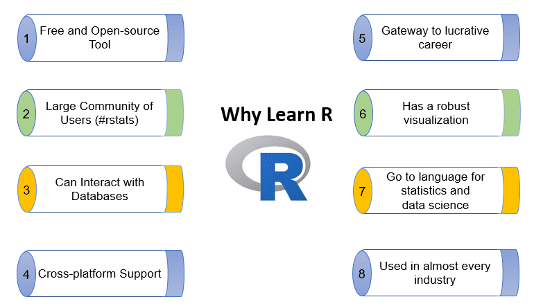
1.4.2 Key Reasons to Learn R

• Free and Open Source: R is entirely free, making it accessible to everyone.

• Extensive Community Support: An active global community constantly develops and shares resources.

• Industry Application: From tech giants like Google and Facebook to finance leaders like JPMorgan and HSBC, R is a trusted tool across industries.

Figure 1.1: Compelling Reasons to Learn R

1.4.3 Companies Using R for Analytics

R’s widespread adoption is evident in the diversity of industries leveraging its capabilities. From creating predictive models to visualising business trends, companies like Facebook, Google, Deloitte, and HSBC rely on R for analytics.

Figure 1.2: Major Companies Using R Programming

For instance, data analysts at Netflix use R to understand viewing patterns and recommend shows to users. Healthcare professionals employ R to analyse patient data for better treatment outcomes. By learning R, you’re gaining a skill that is in demand across various industries.

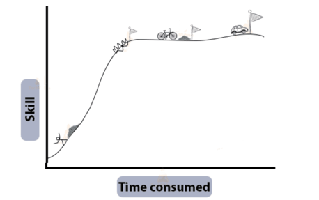
1.4.4 A Steep Yet Rewarding Learning Curve

R’s learning curve can be steep initially. However, its design makes once-difficult tasks easier and intuitive. As you progress, you will automate complex workflows, create visually compelling graphics, and perform advanced analyses efficiently.

Figure 1.3: The Learning Curve of R Programming

1.5 Experiment 1.1: Installing R and RStudio

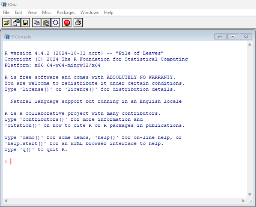
R is the core programming language (Figure 1.4 (a)), while RStudio is an integrated development environment (IDE) that facilitates writing, executing, and debugging R code (Figure 1.4 (b)).

(a) R Graphical User Interface (Rgui)

(b) RStudio Interface

Figure 1.4: Comparing the R GUI and RStudio IDE Interfaces

1.5.1 Installing R

The installation process for R varies slightly depending on your operating system:

• For Windows Users:

  Visit the CRAN (Comprehensive R Archive Network) website at this link. Download the latest version of R for Windows, then follow the installation prompts to complete the setup.

• For Mac Users:

  Visit the CRAN website for Mac at this link. Download the appropriate version for your macOS, and follow the on-screen instructions to install it.

1.5.2 Installing RStudio

Once R is installed, you should install RStudio, which provides an easier interface for interacting with R.

• Visit the RStudio download page. Select the free version of RStudio Desktop, and download the appropriate installer for your operating system (Windows, macOS, or Linux). Then, run the installer and follow the instructions.

Code Execution Guidance

After installing R and RStudio, open RStudio to ensure everything works correctly. The R console will appear in the lower-left pane, indicating that R is ready to use.

With R and RStudio installed you’re ready to start your journey into data analysis, statistical computing, and programming with R!

1.5.3 Practice Quiz 1.1

Question 1:

What is the primary role of R in the R programming environment?

1. A user interface for writing code
   
2. A programming language for statistical computing
   
3. A package manager
   
4. A data visualization tool

Question 2:

Which of the following best describes RStudio?

1. A standalone programming language
   
2. A text editor for writing R scripts
   
3. An Integrated Development Environment (IDE) for R
   
4. A package repository for R

Question 3:

Which of the following is the correct sequence of steps to install R and RStudio on your computer?

1. Install RStudio first, then install R from the CRAN website.
   
2. Install R from the CRAN website first, then install RStudio.
   
3. Download both R and RStudio from the RStudio website and install them simultaneously.
   
4. Install R from the Microsoft Store, then install RStudio from the CRAN website.

Question 4:

Which keyboard shortcut runs the current line of code in RStudio on Windows?

1. Ctrl + S
   
2. Ctrl + Enter
   
3. Alt + R
   
4. Shift + Enter

Question 5:

After successful installation, which pane in RStudio indicates that R is ready to use?

1. Source Pane
   
2. Console Pane
   
3. Environment Pane
   
4. Files Pane

See the Solution to Quiz 1.1

1.6 Experiment 1.2: Exploring the RStudio Interface

Now that you have R and RStudio installed let’s explore the RStudio interface. Understanding the layout and purpose of each pane will help you navigate and use RStudio effectively.

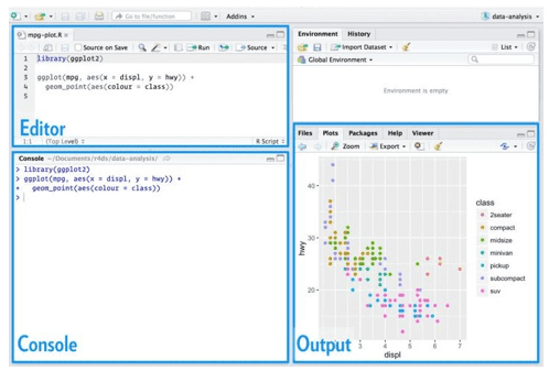
1.6.1 The Four Panes of RStudio

RStudio is divided into four main panes, each serving a specific purpose to enhance your coding workflow².

Figure 1.5: Annotated Overview of Key RStudio Panels

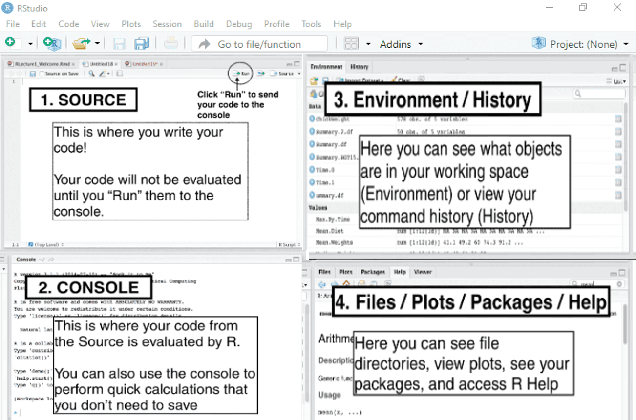
1.6.1.1 Source Pane

• This is where you write your R code. Think of it as your notepad or a place to draft your work.

• The code you write here won’t run until you specifically tell it to. You do this by clicking the “Run” button or using the keyboard shortcut (Ctrl + Enter for Windows or Cmd + Enter for Mac).

• The Source Pane is excellent for writing scripts you can save and use later.

1.6.1.2 Console Pane

• This is the heart of R’s interaction with you. It’s where R evaluates your commands.

• When you “Run” your code from the Source, it appears here, and R processes it immediately.

• You can also directly type commands here for quick calculations or testing. However, anything you type in the console won’t be saved if you close RStudio.

1.6.1.3 Environment/History Pane

• Environment Tab: This shows all the variables, data frames, and objects you’ve created in your current R session. It’s like a snapshot of everything you’re working with.

• History Tab: This records every command you’ve entered, allowing you to track your actions.

1.6.1.4 Files/Plots/Packages/Help Pane

• Files Tab: View and manage the files on your computer, similar to a file explorer.

• Plots Tab: Displays any graphs or charts you create with your R code.

• Packages Tab: Shows the packages (additional tools and functions) available in R and allows you to install, load, or update them as needed.

• Help Tab: This is your go-to place for understanding how functions work. If you’re unsure about something, R’s built-in documentation will be here to guide you.

How to Run Code in RStudio

To execute the code in the Source Pane:

1. Place your cursor on the line of code you want to run.

2. Press Ctrl + Enter (Windows) or Cmd + Enter (Mac) to run the current line.

3. To run multiple lines, highlight the code block and use the same shortcut.

4. Observe the output in the Console Pane.

This practice will help you test code snippets as you progress through the lab.

1.6.2 Performing Basic Calculations in R

R is a powerful and versatile tool for performing all standard arithmetic operations. It supports a range of basic operators, including Addition (+), Subtraction (-), Multiplication (*), Division (/), Exponentiation (^ or **), Modulo (%%), and Parentheses (()), which allow for grouping operations to enforce precedence.

Table 1.1 below summarizes the basic arithmetic operations in R, including their mathematical symbols, corresponding R operators, examples, and results.

Table 1.1: Arithmetic Operations in R: Symbols, Operators, and Examples

Arithmetic Operations	Mathematical Symbol	R Operator	Examples	Result
Addition	+	+	3 + 2	5
Subtraction	-	-	3 - 1	2
Multiplication	×	*	3 * 2	6
Division	÷	/	4 / 2	2
Exponentiation	\(a^b\)	^ or **	2 ^ 2 or 2 ** 2	4
Parentheses	( )	( )	2 * (2 + 1)	6
Modulus	3 mod 2	%%	3 %% 2	1

Examples:

Here are examples of basic arithmetic operations in R:

6 + 12 - 8 # Performs addition and subtraction

#> [1] 10

2 * 3 # Multiplies two numbers

#> [1] 6

100 / 50 # Divides 100 by 50

#> [1] 2

3 * 5 / 3 # Combines multiplication and division

#> [1] 5

3^2 # Raises 3 to the power of 2 (can also use 3**2)

#> [1] 9

Modulo Operation

The modulus (or “mod”) operator returns the remainder after division. For example, 9 mod 2 = 1 because dividing 9/2 = 4 leaves a remainder of 1. In R, this is written as:

9 %% 2 # Returns 1

#> [1] 1

Parenthesis or brackets

Parentheses are used to group operations and override the default precedence of operators. In mathematics, you may know this as BODMAS (Brackets, Orders, Division, Multiplication, Addition, Subtraction). In programming, we use BEDMAS: Brackets, Exponentiation, Division, Multiplication, Addition, Subtraction.

For example:

3 * (2 + 3) # Evaluates (2 + 3) first, then multiplies the result by 3

#> [1] 15

(3 + 2) * (6 - 4) # Groups operations with parentheses

#> [1] 10

Square Root Calculations

Use the sqrt() function to calculate square roots,. For example:

sqrt(125)

#> [1] 11.18034

You can also combine square roots with other operations:

19 / sqrt(19)

#> [1] 4.358899

1.6.3 Comments in R

Comments in R begin with the # symbol and are ignored during execution. They are essential for:

1. Making your code easier to understand.

2. Helping others interpret your code.

3. Documenting your thought process.

Example:

# Multiplying 2 by 8

2 * 8

#> [1] 16

It is a good practice to add a space after the # for better readability:

3 + 6 # Adding 3 and 6

#> [1] 9

1.6.4 Comparison Operators

Comparison operators compare values and return TRUE or FALSE, known as logical. The following are the most common comparison operators in R:

• Equal to (==)

• Not equal to (!=)

• Greater than (>)

• Less than (<)

• Greater than or equal to (>=)

• Less than or equal to (<=)

5 == 3 # Returns FALSE

#> [1] FALSE

25 != 10 # Returns TRUE

#> [1] TRUE

100 > 30 # Returns TRUE

#> [1] TRUE

60 >= 45 # Returns TRUE

#> [1] TRUE

100 <= 1000 # Returns TRUE

#> [1] TRUE

Common Errors and Debugging Tips

• Syntax Errors: Missing commas, unmatched parentheses, or misspelt functions can cause errors.

• Tip: Read error messages carefully; they often indicate the line number and type of error.

• Incorrect Operator Use: Using = instead of == for comparison.

• Tip: Remember that = is for assignment, == is for comparison.

1.6.5 Practice Quiz 1.2

Question 1:

Which pane in RStudio is primarily used for writing and editing R scripts?

1. Console Pane
   
2. Source Pane
   
3. Environment Pane
   
4. Files Pane

Question 2:

What does the Environment Tab in RStudio display?

1. Available packages and their statuses
   
2. Active variables, data frames, and objects in the current session
   
3. The file directory of your project
   
4. Graphical plots and visualizations

Question 3:

How can you execute a selected block of code in the Source Pane?

1. Press Ctrl + S
   
2. Press Ctrl + Enter
   
3. Click the “Run” button
   
4. Both b) and c)

Question 4:

Which pane would you use to install and load R packages?

1. Source Pane
   
2. Console Pane
   
3. Files Pane
   
4. Packages Tab within Files/Plots/Packages/Help Pane

Question 5:

Where can you find R’s built-in documentation and help files within RStudio?

1. Source Pane
   
2. Console Pane
   
3. Environment Pane
   
4. Help Tab within Files/Plots/Packages/Help Pane

See the Solution to Quiz 1.2

1.6.6 Exercise 1.2.1: Basic Calculations

• Explore RStudio

  Open RStudio and familiarise yourself with the four panes.

• Perform Calculations

  Perform the following calculations in the Source Pane, adding comments where appropriate:

  • \(2 + 6 -12\)

  • \(4 \times 3 - 8\)

  • \(81\div 6\)

  • \(16 \text{ mod } 3\)

  • \(2^3\)

  • \((3 + 2) \times (6 - 4) + 2\)

See the Solution to Exercise 1.2.1

1.7 Experiment 1.3: Understanding Atomic Data Types and Variable Assignment

Now that you’re comfortable using R for basic arithmetic and understand how to write comments and use comparison operators, let’s delve into how R handles different data types. In this section, we’ll explore atomic data types and learn how to assign values to variables, which are fundamental concepts in programming.

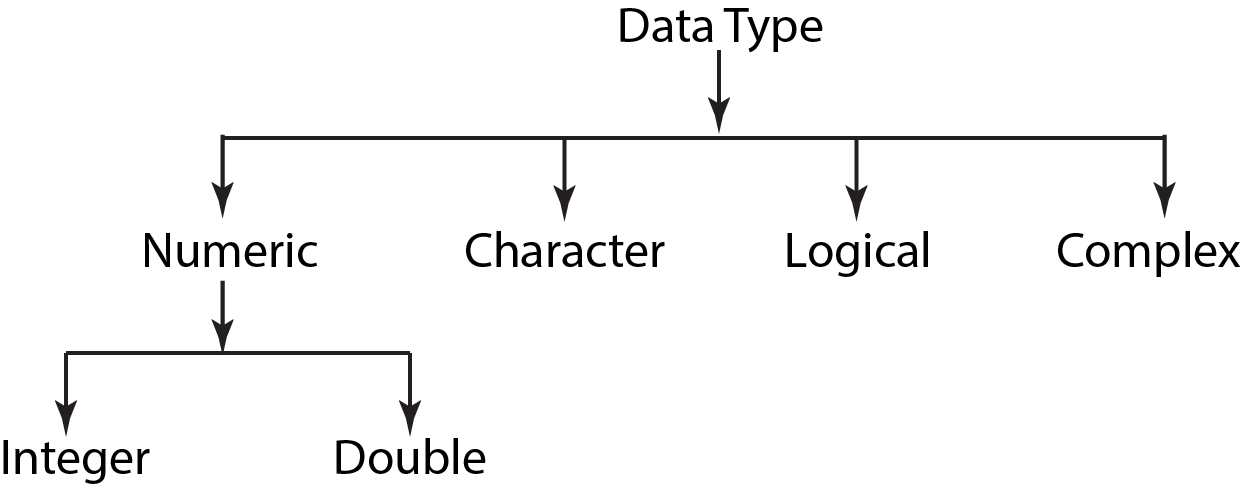
1.7.1 Atomic Data Types

R works with several atomic data types:

• Numeric: Integers (e.g., 4, -2) or doubles (e.g., 4.7, -0.26)

• Character: Text strings enclosed in quotes (e.g., "Nigeria", "Hello world")

• Logical: Boolean values (TRUE, FALSE)

• Complex: Represents numbers with real and imaginary parts (e.g., 2 + 3i, -1.5 - 4i).

Figure 1.6: Data Types in R Programming

You can determine the data type of an object using the class() function.

class(2) # Returns "numeric"

#> [1] "numeric"

class("Anthony Joshua") # Returns "character"

#> [1] "character"

class(TRUE) # Returns "logical"

#> [1] "logical"

class(2 + 3i) # Returns "complex"

#> [1] "complex"

1.7.2 Variable Assignment

When working in R, you’ll often find yourself storing values, results, or objects for later use. This is where variables come in. Variables allow you to hold onto data so that you can reference it easily whenever you need it. Assigning a value to a variable is straightforward in R, and you can do this using the assignment operator, which is <- or =. While both work, you’ll notice that most R users prefer <- for assignments³. This preference is largely based on convention and readability, as it helps keep your code clean and consistent.

Let’s look at a few examples of the variable assignments in action. Here, we’ll assign different types of data to variables.

number <- 10 # 'number' now holds the value 10

class(number) # Returns "numeric"

#> [1] "numeric"

state <- "Lagos"

class(state) # Returns "character"

#> [1] "character"

After running these lines, each variable (number, state) stores a value you can reuse or modify later in your code. For instance, if you want to check the value of number, just type:

number

#> [1] 10

And R will display the stored value.

Tip

If you’re using a Windows, a quick way to type the assignment operator <- is by pressing ALT + _; on a Mac, you can use Option + _. This shortcut can save time as you write and assign variables in R.

Once you’ve assigned a value to a variable, you can use that variable in expressions. For instance:

x <- 15

y <- 12

x + 1

#> [1] 16

x + y

#> [1] 27

It’s also good to know that you can overwrite variables if needed. Say you assigned x <- 15, but later, you decide x should be 20. You can just assign it again:

x <- 20

Now, every time you call x, R will know that its value is 20, not 15 anymore.

1.7.3 Rules for Naming Variables

• Must start with a letter.

• Can contain letters, numbers, underscores _, or dots . after the first letter.

• No spaces or special characters.

• R is case-sensitive (Age and age are different variables).

Best Practices

• Name Your Variables Clearly: Choose names that describe their data, like total_sales or average_height, rather than generic names like x or y. Using clear, descriptive variable names is a best practice because it makes your code easier to understand and maintain. This way, anyone reading your code can quickly grasp the purpose of each variable without needing additional explanations.

• Avoid Overwriting R’s Built-in Functions: Names like mean, sum, and data are already used by R, so avoid using these as variable names to prevent errors.

In short, variable assignment is like giving a shortcut name to a value or a piece of data. Once assigned, you can call on that name whenever needed, making your code easier to follow and maintain. And remember, R is pretty flexible, so don’t worry too much if you make a mistake – you can permanently reassign or update your variables as you go!

1.7.4 Exercise 1.3.1: A Quick Hands-On

Try it yourself! Create a variable named my_name and assign your name to it. Then, print a greeting that says:
Hello, [Your Name]!

See the Solution to Exercise 1.3.1

1.7.5 Reflective Exercise 1.3.2: Best Practices and Pitfalls in Variable Naming

In this exercise, you will explore the differences between acceptable and unacceptable variable names in R. Understanding why some naming conventions work and others don’t is essential for writing clean, error-free code.

Instructions:

1. Review the Table 1.2 below and identify why each name is either acceptable or unacceptable according to R’s variable naming rules.

2. Answer the following questions:

   • Why are some variable names acceptable while others are not?
   • What makes the acceptable variable names follow R’s rules and best practices?

3. Reflect on how these rules can help make your code more readable and easier to debug.

Table 1.2: Comparison of Valid and Invalid Variable Names

S/N	Acceptable Variable Names	Unacceptable Variable Names
1	health.status	health(status)
2	covid_19_cases	covid-19-cases
3	budget2024	2024budget
4	sales_price_2024	sales price 2024

1.7.6 Data Type Conversions

In R, data comes in various types, such as numeric, character, logical, and complex. Sometimes, you’ll need to convert data from one type to another—a process known as typecasting. This is essential when performing operations requiring data to be in a specific format.

1.7.6.1 Using as. Functions for Typecasting

R provides a set of as. functions that make typecasting straightforward. These functions allow you to explicitly convert variables to a desired data type. Table 1.3 summarising these functions:

Table 1.3: Common Functions to Convert Between Data Types

Data Type Converting To	How to Do It
Numeric	as.numeric(variable_name)
Character	as.character(variable_name)
Logical	as.logical(variable_name)
Complex	as.complex(variable_name)

Example: Converting Character to Numeric

Suppose you have a variable weight that is currently a character string:

weight <- "64.45"

class(weight) # Returns "character"

#> [1] "character"

To perform numerical operations on weight, you need to convert it to a numeric type:

weight_num <- as.numeric(weight)

class(weight_num) # Returns "numeric"

#> [1] "numeric"

Now, weight_num is of numeric type, and you can use it in arithmetic calculations:

weight_num * 2

#> [1] 128.9

1.7.6.2 Handling NA Results

Sometimes, R cannot convert a value to the desired type. When this happens, it returns NA (Not Available) and a warning message. This often occurs in the following situations:

• Converting Non-Numeric Characters to Numeric: If a character string contains letters or symbols that cannot be interpreted as numbers.

• Converting Non-Boolean Strings to Logical: If the string does not represent TRUE or FALSE.

Example 1:

height <- "161.5 cm"

as.numeric(height) # Returns NA with a warning

#> Warning: NAs introduced by coercion

#> [1] NA

In this case, the string "161.5 cm" includes non-numeric characters (" cm"), so R cannot convert it to a numeric value.

Example 2:

smiling_face <- "No"

as.logical(smiling_face)

#> [1] NA

Here, "No" does not correspond to TRUE or FALSE, so the conversion fails.

Common Errors and Debugging Tips

• NA Values After Conversion: Occurs when non-numeric characters are present in a string being converted to numeric.

• Tip: Clean your data to ensure it contains only the characters you expect.

• Variable Not Found: This occurs when you try to use a variable that hasn’t been defined.

• Tip: Ensure you’ve assigned a value to the variable and that it’s spelled correctly.

Best Practices

• Inspect Your Data: Before converting, check your data to ensure it’s in the correct format.

• Handle NAs Appropriately: Use functions like is.na() to identify and manage NA values after conversion.

• Clean Data When Necessary: Remove or replace unwanted characters that may prevent successful conversion.

By understanding how to perform data type conversions and handle potential issues, you’ll be better equipped to manipulate and analyze data effectively in R.

1.7.7 Practice Quiz 1.3

Question 1:

Which function is used to determine the class of an object in R?

1. vector()
   
2. c()
   
3. class()
   
4. typeof()

Question 2:

What will the class of the following object be in R?

my_var <- TRUE

1. numeric
   
2. character
   
3. logical
   
4. complex

Question 3:

Which of the following is an acceptable variable name in R?

1. 2nd_place
   
2. total-sales
   
3. average_height
   
4. user name

Question 4:

How can you convert a character string "123" to a numeric type in R?

1. to.numeric("123")
   
2. as.numeric("123")
   
3. convert("123", "numeric")
   
4. numeric("123")

Question 5:

What will be the result of the following R code?

weight <- "60.4 kg"
weight_numeric <- as.numeric(weight)

1. 60.4
   
2. "60.4"
   
3. NA with a warning
   
4. NULL

See the Solution to Quiz 1.3

1.7.8 Exercise 1.3.3: Variable Assignment and Data Types

Determine the classes of the following variables and convert them if necessary. Fill in the blanks (indicated by ---) to complete the code.

age <- 15

---(age) # What is the class?

weight <- "60.4 kg"

class(---)  # What is the class?

# Can you convert weight to numeric?
weight_numeric <- ---(weight)

smile_face <- "FALSE"

---(smile_face)  # What is the class?

# What happens if you convert smile_face to logical?
smile_face_logical <- as.logical(---)

See the Solution to Exercise 1.3.3

Common Errors and Debugging Tips

• Converting Strings with Units: Direct conversion may fail due to non-numeric characters.

• Tip: Use gsub() to remove unwanted characters before conversion.

1.8 Experiment 1.4: Conditional Statements in R

Conditional statements are a vital tool for controlling the flow of your program based on logical conditions. They allow you to execute different blocks of code depending on whether certain conditions are true or false, making your code dynamic and adaptable. The primary constructs are if, else, else if.

Figure 1.7: If-Else Statement in R Programming

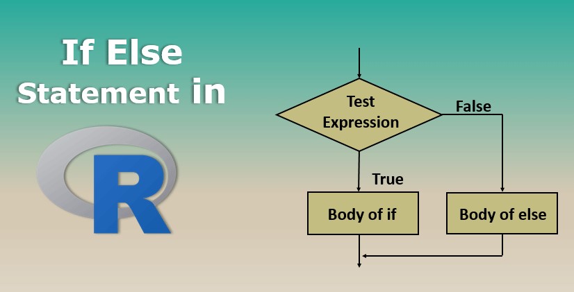
1.8.1 The if Statement

This is the most basic conditional construct. It executes code only if a specified condition is TRUE.

x <- 5
if (x > 3) {
  print("x is greater than 3")
}

#> [1] "x is greater than 3"

1.8.2 The else Statement

Provides an alternative set of instructions if the if condition is FALSE.

x <- 2
if (x > 3) {
  print("x is greater than 3")
} else {
  print("x is not greater than 3")
}

#> [1] "x is not greater than 3"

1.8.3 The else if Statement

The else if can be used to check situations with multiple conditions sequentially. It provides an additional condition check after the initial if statement.

x <- 3
if (x > 5) {
  print("x is greater than 5")
} else if (x == 5) {
  print("x is equal to 5")
} else {
  print("x is less than 5")
}

#> [1] "x is less than 5"

Using Logical Operators

You can combine conditions using logical operators:

• AND (&): Both conditions must be TRUE.
• OR (|): At least one condition must be TRUE.
• NOT (!): Inverts the logical value.

Example using AND (&):

x <- 8
y <- 12

if (x < 10 & y > 10) {
  print("Both conditions are true")
} else {
  print("At least one condition is false")
}

In this example, the if statement checks if both x < 10 and y > 10 are TRUE. Since both conditions are TRUE, the output will be:

"Both conditions are true"

Example using OR (|):

a <- 3
b <- 20

if (a < 5 | b > 25) {
  print("At least one condition is true")
} else {
  print("Neither condition is true")
}

In this example, the if statement checks if either a is less than 5 or b is greater than 25. Since a < 5 is TRUE, the output will be: 

"At least one condition is true"

Example using NOT (!):

c <- FALSE

if (!c) {
  print("The condition is false")
} else {
  print("The condition is true")
}

Here, the if statement uses the NOT operator to check if c is not TRUE. Since c is FALSE, !c becomes TRUE, and the output will be:

"The condition is false"

1.8.4 The ifelse() Function

The ifelse() function is a vectorised form of conditional statements. It applies a condition to each element of a vector and returns one value if the condition is TRUE and another value if the condition is FALSE. The syntax is as follows:

ifelse(condition, value_if_true, value_if_false)

Where:

• condition: A logical expression to evaluate.

• value_if_true: The value to return if the condition is TRUE.

• value_if_false: The value to return if the condition is FALSE.

Example:

number <- 21

ifelse(number %% 2 == 0, "Even", "Odd")

#> [1] "Odd"

In this example, ifelse() checks whether number %% 2 == 0 (that is, whether number is even). If it is even, it returns "Even"; otherwise, it returns "Odd". For more advanced uses, see Chapter 2.5.5.5.

1.8.5 The switch Function

The switch() function is a control flow statement that allows you to execute different pieces of code based on the value of an expression. It’s particularly useful when you have multiple conditions to check and want a cleaner alternative to lengthy if...else statements.

There are two primary ways to use switch() in R:

1. Numeric Switching: Where the expression evaluates to a numeric index.

2. Character Switching: Where the expression evaluates to a character string matching one of the named alternatives.

The general structure of switch() function is as follows:

switch(EXPR,
  ...
)

Where:

• EXPR: An expression that evaluates to a numeric value or a character string.

• ...: A sequence of alternatives (unnamed or named arguments).

The switch() function uses the same syntax for both numeric and character expressions. The behavior of the function depends on the type of the EXPR argument you provide.

When to Use switch()

• When you have a variable that can take on multiple known values and you want to execute different code based on each value.

• To improve code readability over multiple if...else statements.

• When performance is a consideration, as switch() can be more efficient than multiple if...else checks.

Example 1: Day of the Week Activities Using Character Switching

Suppose you want to plan activities based on the day of the week.

day <- "Saturday"

activity <- switch(day,
  Monday = "Go to the gym",
  Tuesday = "Attend a cooking class",
  Wednesday = "Work from home",
  Thursday = "Meet friends for dinner",
  Friday = "Watch a movie",
  Saturday = "Go hiking",
  Sunday = "Rest and recharge",
  "Invalid day"
)

print(paste("Today's activity:", activity))

#> [1] "Today's activity: Go hiking"

Explanation

• Variable day: Contains the day of the week as a string.

• Using switch():

  • Matches day against the provided day names.

  • If a match is found, returns the corresponding activity.

  • If no match is found, returns "Invalid day".

Example 2: Mapping Codes to Descriptions Using Character Switching

Suppose you have status codes that need to be mapped to descriptive messages.

status_code <- 404

message <- switch(as.character(status_code),
  "200" = "OK: The request has succeeded.",
  "301" = "Moved Permanently: The resource has moved.",
  "400" = "Bad Request: The request could not be understood.",
  "401" = "Unauthorized: Authentication is required.",
  "404" = "Not Found: The resource could not be found.",
  "500" = "Internal Server Error: The server encountered an error.",
  "Unknown Status Code"
)

print(message)

#> [1] "Not Found: The resource could not be found."

Explanation:

• Variable status_code: Contains an HTTP status code.

• Converting to Character: as.character(status_code) because switch() with character matching requires a string.

• Using switch():

  • Matches the status code against the provided cases.

  • Returns the corresponding message or "Unknown Status Code" if no match is found.

Example 3: Simple Calculator Using Numeric Switching

Let’s create a simple calculator that performs operations based on a numeric choice.

# User inputs
num1 <- 10
num2 <- 5
# Options: 1 for addition, 2 for subtraction, 3 for multiplication, 4 for division
choice <- 3

# Use switch() to perform the selected operation
result <- switch(choice,
  num1 + num2, # If choice == 1
  num1 - num2, # If choice == 2
  num1 * num2, # If choice == 3
  if (num2 != 0) num1 / num2 else "Division by zero error", # If choice == 4
  "Invalid operation"
) # Default if choice > number of cases

# Display the result
print(paste("The result is:", result))

#> [1] "The result is: 50"

Explanation

• Variables:

  • num1, num2: Numbers to operate on.

  • choice: Numeric choice of operation.

• Using switch():

  • Since choice is numeric, switch() selects the expression based on position.

    • 1: num1 + num2

    • 2: num1 - num2

    • 3: num1 * num2

    • 4: Division with a check for division by zero.

  • If choice exceeds the number of provided alternatives (4), the default "Invalid operation" is returned.

Common Errors and Debugging Tips

• Missing Braces {}: Forgetting to include braces in if statements.

• Tip: Always include braces even if there’s only one line of code inside.

• Incorrect Logical Operators: Using && instead of & or || instead of | can lead to unexpected results.

• Tip: Use & and | for vectorized operations, which is common in R.

1.8.6 Practice Quiz 1.4

Question 1:

What will be the output of the following R code?

number <- 10
if (number %% 2 == 0) {
  print("Even")
} else {
  print("Odd")
}

1. Odd
   
2. Even
   
3. TRUE
   
4. FALSE

Question 2:

Which logical operator in R returns TRUE only if both conditions are TRUE?

1. | (OR)
   
2. & (AND)
   
3. ! (NOT)
   
4. ^ (XOR)

Question 3:

In the switch() function, what does the following code return when choice is 3?

num1 <- 10
num2 <- 5
choice <- 3

result <- switch(choice,
  num1 + num2,
  num1 - num2,
  num1 * num2,
  "Invalid operation"
)

print(result)

1. 15
   
2. 5
   
3. 50
   
4. "Invalid operation"

Question 4:

What is the purpose of including a default case in a switch() statement?*

1. To handle cases where the expression matches multiple conditions
   
2. To execute a block of code if none of the specified cases match
   
3. To prioritize certain cases over others
   
4. To initialize variables within the switch

Question 5:

Which of the following uses the NOT (!) operator correctly in an if statement?

if (!c) {
  print("The condition is false")
}

if (c!) {
  print("The condition is false")
}

if (c != TRUE) {
  print("The condition is false")
}

4. Both a) and c)

See the Solution to Quiz 1.4

1.8.7 Exercise 1.4.1: Conditional Statements

Task 1

What is the output of the following code?

number <- 10

if (number %% 2 == 0) {
  print("Even")
} else {
  print("Odd")
}

Task 2

Given m <- 5 and n <- 7, write code that prints:

• “m is greater than n” if m > n
• “m is less than n” if m < n
• “m and n are equal” if m == n

See the Solution to Exercise 1.4.1

1.8.8 Exercise 1.4.2: Menu Selection Using switch()

Simulate a simple text-based menu where a user selects an option. Use the switch() function to determine the action based on the user’s selection.

Your Task:

1. Simulate User Input:

   • Assign a value to a variable option to represent the user’s selection.

   • Possible options: "balance", "deposit", "withdraw", "exit".

2. Use the switch() Function:

   • Match the value of option to the appropriate case using switch().

   • For each case, assign a message that describes the action.

Possible Options and Messages:

• “balance”: Display “Your current balance is $1,000.”

• “deposit”: Display “Enter the amount you wish to deposit.”

• “withdraw”: Display “Enter the amount you wish to withdraw.”

• “exit”: Display “Thank you for using our banking services.”

• Default: Display “Invalid selection. Please choose a valid option.”

3. Include a Default Case:
   • If the user input does not match any of the specified options, provide a default message indicating an invalid selection.
4. Display the Message:
   • Use print() to display the message corresponding to the user’s selection.

Here’s a starting point for your code:

# Simulate user input
option <- "---"  # Options could be "balance", "deposit", "withdraw", "exit"

# Use switch() to determine the action
message <- switch(...,
                  balance = "You have $1,000 in your account.",
                  deposit = ...,
                  withdraw = "How much would you like to withdraw?",
                  "Invalid selection. Please choose a valid option.")

# Display the message
print(...)

Replace the ... with the correct values and complete the exercise!

See the Solution to Exercise 1.4.2

1.8.9 Exercise 1.4.3: Mini-Project - Basic Calculator in R

Using what you’ve learned about arithmetic operations, variables, and conditional statements, create a simple calculator program in R that:

• Prompts the user to enter two numbers.

• Asks the user to choose an operation: addition, subtraction, multiplication, or division.

• Performs the operation and displays the result.

Hint:

• Use the readline() function to get user input.

• Convert the input to numeric using as.numeric().

• Use a switch() statement to handle the operation selection.

See the Solution to Exercise 1.4.3

1.9 Further Reading

To further enhance your R programming skills, here are some excellent resources:

• RStudio Cheat Sheets:
  https://www.rstudio.com/resources/cheatsheets

• Introduction to R by RStudio:
  https://education.rstudio.com/learn/beginner

• YaRrr! The Pirate’s Guide to R by Nathaniel D. Phillips
  https://bookdown.org/ndphillips/YaRrr

• R for Data Science by Hadley Wickham, Mine Çetinkaya-Rundel, and Garrett Grolemund
  https://r4ds.hadley.nz

• R for Data Science: Exercise Solutions by Jeffrey B. Arnold
  https://jrnold.github.io/r4ds-exercise-solutions

• Big Book of R by Oscar Baruffa
  https://www.bigbookofr.com

1.10 Reflective Summary

Congratulations on completing Lab 1! You’ve taken your first steps into R programming and have covered much ground:

• Installed R and RStudio
  Set up your programming environment.

• Explored the RStudio Interface
  Learned how to use RStudio’s four main panes to write, execute, and manage your R code effectively.

• Performed Basic Calculations in R
  Practiced using R for arithmetic operations and understood operator precedence.

• Understood Atomic Data Types and Variable Assignment
  Explored numeric, character, and logical data types, and learned how to identify and convert between them.

• Used Conditional Statements in R
  Controlled the flow of your programs using if, else if, and else statements, and used logical operators.

Take a moment to reflect on how these foundational skills can be applied to solving real-world problems. As you progress through this book, each lab will build on these essentials, guiding you toward proficiency in data analysis with R.

Keep experimenting with the code and exploring built-in functions. The more you practice, the more confident and comfortable you’ll become.

What’s Next?

In the next lab, we’ll delve into R’s fundamental data structures, including vectors, matrices, and data frames—key data manipulation and analysis tools.

---

1. For a detailed breakdown of R’s development, refer to the comprehensive timeline created by Tim Brock, Colin Gillespie, and the Jumping Rivers team at https://www.jumpingrivers.com/blog/r-timeline.

2. For a detailed overview of all RStudio’s features, see the RStudio User Guide at https://docs.posit.co/ide/user.

3. You might wonder why R uses <- instead of the = symbol that you might see in other programming languages. While you can use = for assignment in R, it’s generally preferred to use <- for clarity. This is partly because = is also used in function arguments, so sticking to <- makes your code easier to read and helps avoid confusion.