5  Data Transformation

5.1 Introduction

Welcome to Lab 5! In this lab, we will focus on one of the most important steps in the data analysis process: data transformation. Real-world data rarely arrives in perfect, analysis-ready form. Before generating insights, visualising patterns, or constructing models, we must transform the data: cleaning, reshaping, and summarising it into a more meaningful structure.

In this lab, we will explore:

• The native pipe operator |> to create a smooth, readable pipeline of data operations.

• The core dplyr verbs—select(), filter(), mutate(), arrange(), and summarise()—to efficiently manipulate and refine your data.

• Strategies for grouping and summarising data to extract patterns and trends.

• Techniques for identifying and handling missing values responsibly.

These transformations form a vital step in any data workflow, ensuring that your datasets are well-prepared for subsequent analysis or visualisation.

5.2 Learning Objectives

By the end of this lab, you will be able to:

• Streamline Your Code Using the Pipe Operator |>
  Connect multiple data operations into a logical sequence, enhancing code readability and reducing nesting complexity.

• Perform Key Data Transformation Tasks Using dplyr
  Utilise functions like select(), filter(), arrange(), mutate(), and summarise() toreshape, refine, and improve datasets for analysis.

• Gain Insights Through Summarisation and Grouping
  Group data and apply aggregation functions to extract meaningful summaries and trends.

• Handle and Impute Missing Data
  Identify missing values in your datasets, understand their impact, and apply suitable strategies (e.g., removal, mean/median imputation) to maintain data integrity.

• Prepare Data for Analysis and Visualisation
  Clean and structure your datasets so they are ready for modelling, plotting, and communicating results effectively.

By completing this lab, you will master data transformation and become more confident in dealing with messy, real-world datasets and advancing towards deeper analyses.

5.3 Prerequisites

Before starting this lab, you should have:

• Completed Lab 4 or have a solid understanding of organising R projects and managing packages.

• Familiarity with loading data into R and conducting basic data checks (e.g., using glimpse(), head()).

• Interest in refining data, ensuring it is tidy, structured, and ready for more advanced analyses.

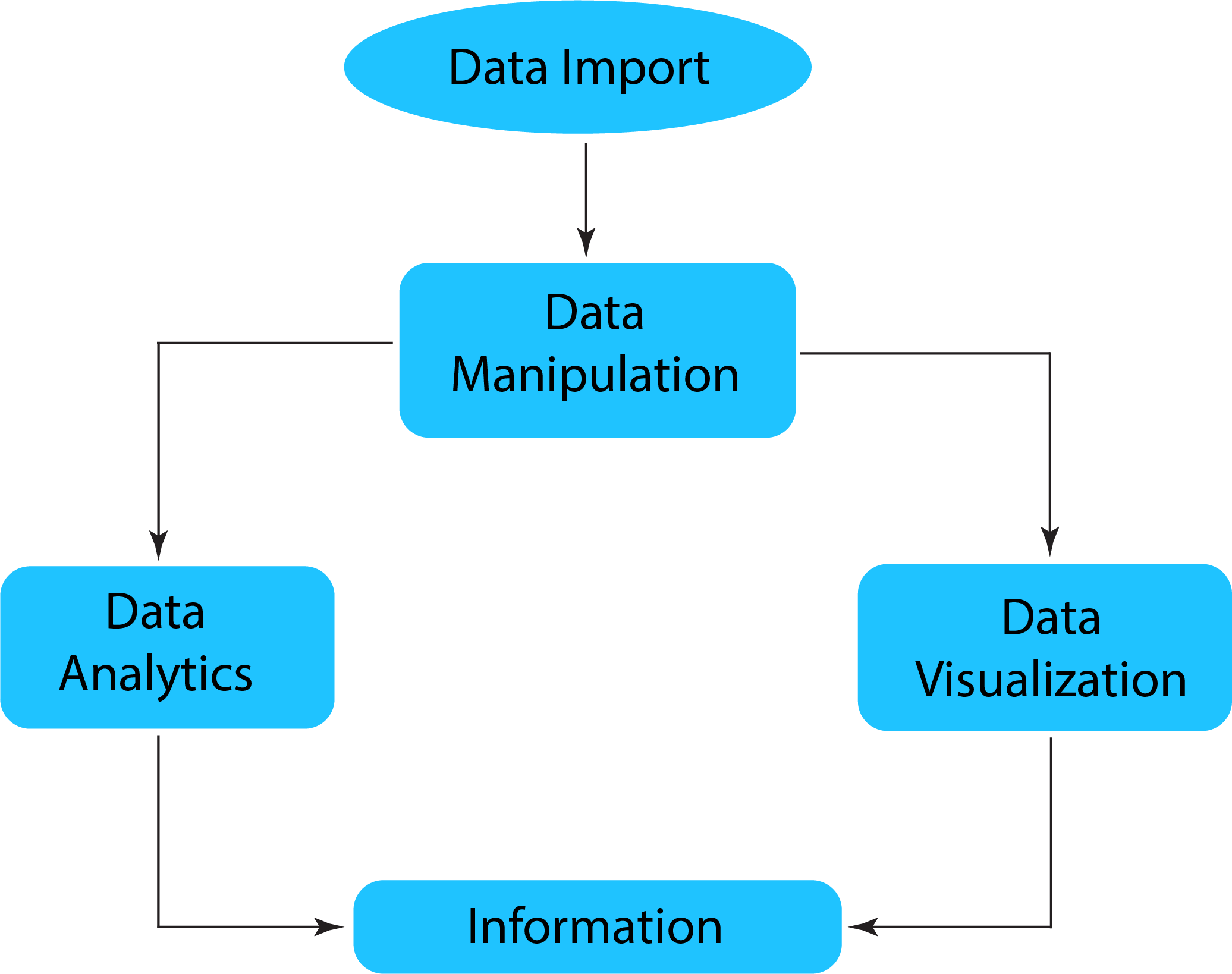
5.4 What is Data Transformation?

Data transformation is the process of reshaping raw data into a more useful format. Real-world data is rarely perfect for immediate analysis. It often contains extra variables, missing values, or is structured in a way that is not conducive to answering your research questions. Data transformation includes:

• Selecting relevant parts of the dataset: Focusing on the rows and columns you actually need.

• Creating new variables: Deriving meaningful metrics from existing data.

• Summarising information: Computing averages, totals, or other aggregate statistics to distil complex information into digestible summaries.

• Organising data into a meaningful structure: Arranging your dataset so that the relationships between variables and observations are clear.

You can think of data transformation like preparing ingredients before cooking: you wash, chop, and measure everything out so that when you start cooking, you can focus on creating your dish without interruptions or confusion.

5.5 Real-World Scenario: Preparing Data for Analysis

Imagine that you work as a data analyst at a wildlife research centre. You have received a raw dataset containing information on various species: their body measurements, diets, sleep patterns, and more. Before you can analyse ecological relationships, test hypotheses, or build models, you need to clean and organise this data. Using the techniques in this lab, you can:

• Select only the columns necessary for your investigation.

• Filter out rows that are not relevant to your study.

• Mutate the dataset to create new metrics or correct errors.

• Arrange the rows to highlight the largest or smallest values.

• Summarise the data by group to identify patterns by species or habitat.

• Handle missing values so that they do not distort your findings.

By applying these transformations, you ensure that your data is analysis-ready.

5.6 Experiment 5.1: The Pipe Operator |>

One of the best tools to simplify your R code is the pipe operator. Traditionally, the <%> operator from the magrittr package has been widely used for this purpose. However, starting from R version 4.1.0, R introduced a native pipe operator |>. The pipe operator allows you to chain functions together in a linear, logical sequence, rather than nesting them inside one another. Using pipes makes your code more readable and helps you think through your data transformations step-by-step.

In this lab, we will be using the base pipe operator |>, which functions similarly to the magrittr <%> operator¹. Imagine you have data frame, data, and you want to perform multiple operations on it, such as applying functions foo and bar in sequence. Without a pipe, you might write as:

bar(foo(data))

This is harder to read than:

data |>
  foo() |>
  bar()

In the piped version, you start with data, then say “and then apply foo(),” and then “and then apply bar(),” which feels more intuitive and mirrors how we naturally describe processes in words.

How to configure native pipe operator

To configure RStudio to insert the base pipe operator |> instead of %>% when pressing Ctrl/Cmd + Shift + M, navigate to the Tools menu, select Global Options…, then go to the Code section. In the Code options, check the box labelled Use native pipe operator, |> (requires R 4.1+).

Figure 5.1: To insert |>, make sure the “Use native pipe operator” option is checked

How Does the Pipe Operator Work?

The pipe operator |> takes the output of one function and passes it as the first argument to the next function.

Example 1

For instance, consider:

iris |> head()

#>   Sepal.Length Sepal.Width Petal.Length Petal.Width Species
#> 1          5.1         3.5          1.4         0.2  setosa
#> 2          4.9         3.0          1.4         0.2  setosa
#> 3          4.7         3.2          1.3         0.2  setosa
#> 4          4.6         3.1          1.5         0.2  setosa
#> 5          5.0         3.6          1.4         0.2  setosa
#> 6          5.4         3.9          1.7         0.4  setosa

This is exactly the same as:

head(iris)

#>   Sepal.Length Sepal.Width Petal.Length Petal.Width Species
#> 1          5.1         3.5          1.4         0.2  setosa
#> 2          4.9         3.0          1.4         0.2  setosa
#> 3          4.7         3.2          1.3         0.2  setosa
#> 4          4.6         3.1          1.5         0.2  setosa
#> 5          5.0         3.6          1.4         0.2  setosa
#> 6          5.4         3.9          1.7         0.4  setosa

Example 2:

Here’s another example combining multiple functions:

x <- 4.234

x |>
  sqrt() |>
  log() |>
  round(2)

#> [1] 0.72

This sequence is equivalent to the nested version:

x <- 4.234

round(log(sqrt(x)), 2)

#> [1] 0.72

Reflection Question:

How does using the pipe operator enhance clarity, compared to nested function calls, especially when performing multiple operations on the same dataset?

By using pipes, you avoid writing nested code and make the flow of your data transformation much clearer.

5.6.1 Practice Quiz 5.1

Question 1:

What is the primary purpose of the pipe operator (|> or %>%) in R?

1. To run code in parallel.
   
2. To nest functions inside one another.
   
3. To pass the output of one function as the input to the next, improving code readability.
4. To automatically clean missing data.

Question 2:

Consider the following R code snippets:

numbers <- c(2, 4, 6)

# Nested function version:
result1 <- round(sqrt(sum(numbers)))

# Pipe operator version:
result2 <- numbers |> sum() |> sqrt() |> round()

For a new R learner, is the pipe operator version generally more readable than the nested function version?

1. True
2. False

Question 3:

What is the output of the following R code?

result <- c(5, 10, 15) 
result |> mean()

1. 10
   
2. 15
   
3. 5
   
4. 30

Question 4:

Which of the following code snippets correctly uses the pipe operator to apply the sqrt() function to the sum of numbers from 1 to 4?

1. sqrt(sum(1:4))
   
2. 1:4 |> sum() |> sqrt()
   
3. sum(1:4) |> sqrt
   
4. 1:4 |> sqrt() |> sum()

Question 5:

What will be the output of the following code?

result <- letters
result |> head(3)

1. c("a", "b", "c")
   
2. c("x", "y", "z")
   
3. c("A", "B", "C")
   
4. An error is thrown.

See the Solution to Quiz 5.1

5.7 Experiment 5.2: Data Manipulation with dplyr

In data analysis, we often encounter datasets that aren’t in the ideal format for our needs. Data comes in all shapes and sizes, and making sense of it requires effective manipulation. This is where data manipulation becomes essential—a fundamental skill that allows you to transform and summarize data efficiently.

The dplyr package, part of the tidyverse, is designed to make data manipulation in R more approachable, efficient, and intuitive. Think of dplyr as your Swiss Army knife for taming messy datasets. It simplifies tasks like filtering, summarizing, grouping, and transforming data. The best part? Its syntax is easy to read and write, almost like having a conversation with your data.

Why Use dplyr?

• Simplicity: Provides straightforward functions that are easy to learn and remember, lowering the barrier to effective data manipulation.

• Efficiency: Optimized for performance, it handles large datasets swiftly, saving you time and computational resources.

• Readability: Code written with dplyr is often more readable and easier to maintain, which is especially beneficial when collaborating with others or revisiting your own work.

• Integration: Works seamlessly with other tidyverse packages like ggplot2 and tidyr, allowing for a cohesive and efficient data analysis workflow.

Figure 5.2: Data Exploration and Analysis Workflow

Getting Started

First, ensure you have the dplyr package installed and loaded. If you haven’t installed it yet, you can install the tidyverse, which includes dplyr.

# Install the tidyverse package (if not already installed)
install.packages("tidyverse")

# Load the tidyverse package
library(tidyverse)

Core dplyr Verbs

The core functions in dplyr are often referred to as “verbs” because they describe actions you perform on your data:

• select(): Choose variables (columns) based on their names or column positions.

• mutate(): Create new columns or modify existing ones.

• filter(): Select rows based on specific conditions.

• arrange(): Reorder rows based on column values.

• summarise(): Reduce multiple values down to a summary statistic.

• group_by(): Group data by one or more variables for grouped operations.

When summarise() is paired with group_by(), it allows you to get a summary row for each group in the data frame.

Figure 5.3: Key Data Manipulation Functions in dplyr

Additional useful functions include:

• rename(): Rename columns.

• distinct(): Find unique rows.

• count(): Count unique values of a variable.

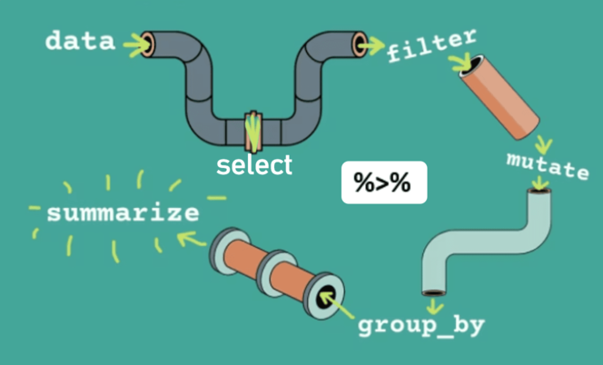
Using Pipes with dplyr functions

One of the key strengths of dplyr is its ability to integrate seamlessly with the pipe operator (%>% or |>), enabling a clean, readable, and intuitive workflow for data manipulation. As illustrated in Figure 5.4, the pipe operator acts as a connector, allowing you to chain multiple dplyr functions in a logical sequence. This approach makes your code easier to read and follow, mirroring the flow of a conversation about your data.

Figure 5.4: Data Transformation Pipeline in dplyr

5.7.1 Working with the dplyr Verbs

Let’s take a deeper dive into each dplyr verb and understand not just how to use them but also what makes them powerful. Remember, the five core verbs—filter(), select(), mutate(), arrange(), and summarize()—are like tools in a toolbox. Each has a specific purpose, but together, they allow you to transform data seamlessly.

Example Datasets

We’ll start our exploration by working with two fascinating datasets: the penguins dataset from the palmerpenguins package² and the msleep dataset from the ggplot2 package. These datasets provide rich, real-world data that will help you practice and apply data manipulation in this book.

1. The penguins Dataset

The penguins dataset³ contains detailed body measurements for 344 penguins from three different species—Adélie, Chinstrap, and Gentoo—found on three islands in the Palmer Archipelago of Antarctica. This dataset includes variables such as:

• Species: The penguin species.

• Island: The island where each penguin was observed.

• Bill Length and Depth: Measurements of the penguin’s bill (beak).

• Flipper Length: The length of the penguin’s flippers.

• Body Mass: The weight of the penguin.

• Sex: The gender of the penguin.

penguins <- palmerpenguins::penguins

penguins |> glimpse()

#> Rows: 344
#> Columns: 8
#> $ species           <fct> Adelie, Adelie, Adelie, Adelie, Adelie, Adelie, Adel…
#> $ island            <fct> Torgersen, Torgersen, Torgersen, Torgersen, Torgerse…
#> $ bill_length_mm    <dbl> 39.1, 39.5, 40.3, NA, 36.7, 39.3, 38.9, 39.2, 34.1, …
#> $ bill_depth_mm     <dbl> 18.7, 17.4, 18.0, NA, 19.3, 20.6, 17.8, 19.6, 18.1, …
#> $ flipper_length_mm <int> 181, 186, 195, NA, 193, 190, 181, 195, 193, 190, 186…
#> $ body_mass_g       <int> 3750, 3800, 3250, NA, 3450, 3650, 3625, 4675, 3475, …
#> $ sex               <fct> male, female, female, NA, female, male, female, male…
#> $ year              <int> 2007, 2007, 2007, 2007, 2007, 2007, 2007, 2007, 2007…

2. The msleep Dataset

Our second dataset, msleep, comes from the ggplot2 package and contains information on the sleep habits of 83 different mammals. This dataset includes 11 variables, such as:

• name: The common name of the mammal.

• genus: The taxonomic genus of the mammal.

• vore: The dietary category of the mammal. Possible values include:

  • "carni": Carnivore (meat-eating)

  • "herbi": Herbivore (plant-eating)

  • "omni": Omnivore (eating both plants and meat)

  • "insecti": Insectivore (eating insects)

• order: The taxonomic order to which the mammal belongs (e.g., Primates, Carnivora).

• conservation: The conservation status of the species, indicating its level of threat or endangerment. Possible values include:

  • "lc": Least Concern

  • "nt": Near Threatened

  • "vu": Vulnerable

  • "en": Endangered

  • "cr": Critically Endangered

  • "domesticated": Domesticated species

• sleep total: Total amount of sleep per day (in hours).

• sleep rem: Amount of REM sleep per day.

• sleep cycle: Length of the sleep cycle.

• awake: The number of hours the mammal spends awake each day (calculated as 24 - sleep_total).

• brain weight: The brain weight of the animal.

• body weight: The body weight of the animal.

msleep <- ggplot2::msleep

msleep |> glimpse()

#> Rows: 83
#> Columns: 11
#> $ name         <chr> "Cheetah", "Owl monkey", "Mountain beaver", "Greater shor…
#> $ genus        <chr> "Acinonyx", "Aotus", "Aplodontia", "Blarina", "Bos", "Bra…
#> $ vore         <chr> "carni", "omni", "herbi", "omni", "herbi", "herbi", "carn…
#> $ order        <chr> "Carnivora", "Primates", "Rodentia", "Soricomorpha", "Art…
#> $ conservation <chr> "lc", NA, "nt", "lc", "domesticated", NA, "vu", NA, "dome…
#> $ sleep_total  <dbl> 12.1, 17.0, 14.4, 14.9, 4.0, 14.4, 8.7, 7.0, 10.1, 3.0, 5…
#> $ sleep_rem    <dbl> NA, 1.8, 2.4, 2.3, 0.7, 2.2, 1.4, NA, 2.9, NA, 0.6, 0.8, …
#> $ sleep_cycle  <dbl> NA, NA, NA, 0.1333333, 0.6666667, 0.7666667, 0.3833333, N…
#> $ awake        <dbl> 11.9, 7.0, 9.6, 9.1, 20.0, 9.6, 15.3, 17.0, 13.9, 21.0, 1…
#> $ brainwt      <dbl> NA, 0.01550, NA, 0.00029, 0.42300, NA, NA, NA, 0.07000, 0…
#> $ bodywt       <dbl> 50.000, 0.480, 1.350, 0.019, 600.000, 3.850, 20.490, 0.04…

Tip

The glimpse() function allows us to quickly view the structure of a data frame in a concise and readable format without printing the entire dataset. It serves as a more user-friendly alternative to the str() function, making it easier to understand the overall composition of your data at a glance.

5.7.2 select() – Picking Specific Columns

The select() function allows you to extract specific columns from a dataset, focusing on only the features relevant to your analysis. It’s like creating a spotlight for just the features you need.

Key Points:

1. Select Columns by Name or Position:

   • You can specify columns by their names or their positions (e.g., 1, 2, 3).

   • This is useful when you only need a few specific columns from a large dataset.

2. Use Helper Functions for Pattern Matching:

   • starts_with("prefix"): Selects columns whose names begin with a specific prefix.

   • ends_with("suffix"): Selects columns whose names end with a specific suffix.

   • contains("substring"): Selects columns whose names contain a specific substring.

3. Deselect Columns Using the Minus (-) Sign:

   • You can drop columns by prefixing their names, indices, or helper functions with -.

   • This is useful when you want to keep most columns but exclude specific ones.

4. Use where() in select():

   • This allows you to select columns programmatically or apply operations to subsets of columns.

5.7.2.1 Selecting Columns by Name:

Suppose we want to extract the name, vore, and sleep_total from the msleep data:

msleep |>
  select(name, sleep_total, vore)

#> # A tibble: 83 × 3
#>    name                       sleep_total vore 
#>    <chr>                            <dbl> <chr>
#>  1 Cheetah                           12.1 carni
#>  2 Owl monkey                        17   omni 
#>  3 Mountain beaver                   14.4 herbi
#>  4 Greater short-tailed shrew        14.9 omni 
#>  5 Cow                                4   herbi
#>  6 Three-toed sloth                  14.4 herbi
#>  7 Northern fur seal                  8.7 carni
#>  8 Vesper mouse                       7   <NA> 
#>  9 Dog                               10.1 carni
#> 10 Roe deer                           3   herbi
#> # ℹ 73 more rows

5.7.2.2 Selecting Columns by Position:

You can use the position of columns to select them, for example, the first three columns:

msleep |>
  select(1:3)

#> # A tibble: 83 × 3
#>    name                       genus       vore 
#>    <chr>                      <chr>       <chr>
#>  1 Cheetah                    Acinonyx    carni
#>  2 Owl monkey                 Aotus       omni 
#>  3 Mountain beaver            Aplodontia  herbi
#>  4 Greater short-tailed shrew Blarina     omni 
#>  5 Cow                        Bos         herbi
#>  6 Three-toed sloth           Bradypus    herbi
#>  7 Northern fur seal          Callorhinus carni
#>  8 Vesper mouse               Calomys     <NA> 
#>  9 Dog                        Canis       carni
#> 10 Roe deer                   Capreolus   herbi
#> # ℹ 73 more rows

5.7.2.3 Selecting Columns Using Patterns:

1. Columns Starting with a Prefix: Select columns starting with “sleep”:

msleep |>
  select(starts_with("sleep"))

#> # A tibble: 83 × 3
#>    sleep_total sleep_rem sleep_cycle
#>          <dbl>     <dbl>       <dbl>
#>  1        12.1      NA        NA    
#>  2        17         1.8      NA    
#>  3        14.4       2.4      NA    
#>  4        14.9       2.3       0.133
#>  5         4         0.7       0.667
#>  6        14.4       2.2       0.767
#>  7         8.7       1.4       0.383
#>  8         7        NA        NA    
#>  9        10.1       2.9       0.333
#> 10         3        NA        NA    
#> # ℹ 73 more rows

2. Columns Ending with a Suffix: Select columns ending with “wt”:

msleep |>
  select(ends_with("wt"))

#> # A tibble: 83 × 2
#>     brainwt  bodywt
#>       <dbl>   <dbl>
#>  1 NA        50    
#>  2  0.0155    0.48 
#>  3 NA         1.35 
#>  4  0.00029   0.019
#>  5  0.423   600    
#>  6 NA         3.85 
#>  7 NA        20.5  
#>  8 NA         0.045
#>  9  0.07     14    
#> 10  0.0982   14.8  
#> # ℹ 73 more rows

3. Columns Containing a Substring: Select columns that contain the word “con”:

msleep |>
  select(contains("con"))

#> # A tibble: 83 × 1
#>    conservation
#>    <chr>       
#>  1 lc          
#>  2 <NA>        
#>  3 nt          
#>  4 lc          
#>  5 domesticated
#>  6 <NA>        
#>  7 vu          
#>  8 <NA>        
#>  9 domesticated
#> 10 lc          
#> # ℹ 73 more rows

5.7.2.4 Deselect Columns Using the Minus Sign:

If you want to keep all columns except name and sleep_total:

msleep |>
  select(-c(name, sleep_total))

#> # A tibble: 83 × 9
#>    genus   vore  order conservation sleep_rem sleep_cycle awake  brainwt  bodywt
#>    <chr>   <chr> <chr> <chr>            <dbl>       <dbl> <dbl>    <dbl>   <dbl>
#>  1 Acinon… carni Carn… lc                NA        NA      11.9 NA        50    
#>  2 Aotus   omni  Prim… <NA>               1.8      NA       7    0.0155    0.48 
#>  3 Aplodo… herbi Rode… nt                 2.4      NA       9.6 NA         1.35 
#>  4 Blarina omni  Sori… lc                 2.3       0.133   9.1  0.00029   0.019
#>  5 Bos     herbi Arti… domesticated       0.7       0.667  20    0.423   600    
#>  6 Bradyp… herbi Pilo… <NA>               2.2       0.767   9.6 NA         3.85 
#>  7 Callor… carni Carn… vu                 1.4       0.383  15.3 NA        20.5  
#>  8 Calomys <NA>  Rode… <NA>              NA        NA      17   NA         0.045
#>  9 Canis   carni Carn… domesticated       2.9       0.333  13.9  0.07     14    
#> 10 Capreo… herbi Arti… lc                NA        NA      21    0.0982   14.8  
#> # ℹ 73 more rows

You can also use helper functions to deselect columns. For instance, drop all columns starting with “sleep”

msleep |>
  select(-starts_with("sleep"))

#> # A tibble: 83 × 8
#>    name                    genus vore  order conservation awake  brainwt  bodywt
#>    <chr>                   <chr> <chr> <chr> <chr>        <dbl>    <dbl>   <dbl>
#>  1 Cheetah                 Acin… carni Carn… lc            11.9 NA        50    
#>  2 Owl monkey              Aotus omni  Prim… <NA>           7    0.0155    0.48 
#>  3 Mountain beaver         Aplo… herbi Rode… nt             9.6 NA         1.35 
#>  4 Greater short-tailed s… Blar… omni  Sori… lc             9.1  0.00029   0.019
#>  5 Cow                     Bos   herbi Arti… domesticated  20    0.423   600    
#>  6 Three-toed sloth        Brad… herbi Pilo… <NA>           9.6 NA         3.85 
#>  7 Northern fur seal       Call… carni Carn… vu            15.3 NA        20.5  
#>  8 Vesper mouse            Calo… <NA>  Rode… <NA>          17   NA         0.045
#>  9 Dog                     Canis carni Carn… domesticated  13.9  0.07     14    
#> 10 Roe deer                Capr… herbi Arti… lc            21    0.0982   14.8  
#> # ℹ 73 more rows

5.7.2.5 Using where() with select()

The where() helper function enables you to dynamically select or modify columns in your data. When used with select(), it allows you to programmatically choose columns based on specific criteria. For example, to select all numeric columns, you can use where(is.numeric):

msleep |>
  select(where(is.numeric))

#> # A tibble: 83 × 6
#>    sleep_total sleep_rem sleep_cycle awake  brainwt  bodywt
#>          <dbl>     <dbl>       <dbl> <dbl>    <dbl>   <dbl>
#>  1        12.1      NA        NA      11.9 NA        50    
#>  2        17         1.8      NA       7    0.0155    0.48 
#>  3        14.4       2.4      NA       9.6 NA         1.35 
#>  4        14.9       2.3       0.133   9.1  0.00029   0.019
#>  5         4         0.7       0.667  20    0.423   600    
#>  6        14.4       2.2       0.767   9.6 NA         3.85 
#>  7         8.7       1.4       0.383  15.3 NA        20.5  
#>  8         7        NA        NA      17   NA         0.045
#>  9        10.1       2.9       0.333  13.9  0.07     14    
#> 10         3        NA        NA      21    0.0982   14.8  
#> # ℹ 73 more rows

5.7.3 mutate() – Creating or Modifying Columns

The mutate() function is like a magic wand for adding new variables or transforming existing ones. Use it whenever you need to derive new information from your dataset.

Key Points:

• You can add as many new columns as you need.

• Existing columns can be modified by overwriting them.

5.7.3.1 Creating a New Column:

Sleep is a vital physiological process, but its duration varies widely among mammals⁴. Understanding how sleep duration relates to body weight could reveal insights into the metabolic and ecological factors influencing sleep. For example:

• Larger mammals may have lower sleep-to-body-weight ratios due to their lower metabolic rates relative to body size.

• Smaller mammals might have higher sleep-to-body-weight ratios, potentially linked to their higher metabolic demands.

To explore this, we calculate the ratio of total sleep (sleep_total) to body weight (bodywt) for each species in the msleep dataset:

msleep |>
  select(name, vore, sleep_total, bodywt) |>
  mutate(sleep_to_weight = sleep_total / bodywt)

#> # A tibble: 83 × 5
#>    name                       vore  sleep_total  bodywt sleep_to_weight
#>    <chr>                      <chr>       <dbl>   <dbl>           <dbl>
#>  1 Cheetah                    carni        12.1  50             0.242  
#>  2 Owl monkey                 omni         17     0.48         35.4    
#>  3 Mountain beaver            herbi        14.4   1.35         10.7    
#>  4 Greater short-tailed shrew omni         14.9   0.019       784.     
#>  5 Cow                        herbi         4   600             0.00667
#>  6 Three-toed sloth           herbi        14.4   3.85          3.74   
#>  7 Northern fur seal          carni         8.7  20.5           0.425  
#>  8 Vesper mouse               <NA>          7     0.045       156.     
#>  9 Dog                        carni        10.1  14             0.721  
#> 10 Roe deer                   herbi         3    14.8           0.203  
#> # ℹ 73 more rows

Tip

This ratio provides a standardised measure to compare sleep duration across species with varying body sizes.

In the same msleep dataset, we suspect that any brain weight greater than 4 is likely an error. To address this, we:

1. Exclude these suspected outliers by replacing them with NA.

2. Retain valid brain weight values for analysis.

msleep |>
  select(name, brainwt) |>
  # Replace brainwt > 4 with NA
  mutate(brainwt_corrected = ifelse(brainwt > 4, NA, brainwt)) |>
  # Sort by original brain weight in descending order
  arrange(desc(brainwt))

#> # A tibble: 83 × 3
#>    name             brainwt brainwt_corrected
#>    <chr>              <dbl>             <dbl>
#>  1 African elephant   5.71             NA    
#>  2 Asian elephant     4.60             NA    
#>  3 Human              1.32              1.32 
#>  4 Horse              0.655             0.655
#>  5 Chimpanzee         0.44              0.44 
#>  6 Cow                0.423             0.423
#>  7 Donkey             0.419             0.419
#>  8 Gray seal          0.325             0.325
#>  9 Baboon             0.18              0.18 
#> 10 Pig                0.18              0.18 
#> # ℹ 73 more rows

Note

1. select(name, brainwt): Focuses on the columns relevant to this analysis: the species’ name and their brain weight.

2. mutate(brainwt_corrected = ifelse(brainwt > 4, NA, brainwt)):

   • Uses ifelse() to create a new column, brainwt_corrected, where any brainwt above 4 is replaced with NA.

   • Values 4 or below remain unchanged.

3. arrange(desc(brainwt)):

   • Sorts the data by the original brainwt in descending order, making it easier to verify the replaced outliers. (You will soon learn more about the arrange() function.)

To better understand patterns in sleep behaviour, it can be helpful to categorize species into discrete groups based on their sleep duration. This makes it easier to group species for further analysis, or explore ecological or evolutionary hypotheses.

For example, we can categorize species as:

• “Long sleepers”: Those that sleep more than 9 hours per day.

• “Short sleepers”: Those that sleep 9 hours or less per day.

We achieve this categorization using the ifelse() function, which allows us to transform the continuous numeric variable sleep_total into a categorical variable, sleep_category.

msleep |>
  select(name, vore, sleep_total) |>
  mutate(sleep_category = ifelse(sleep_total > 9, "long", "short"))

#> # A tibble: 83 × 4
#>    name                       vore  sleep_total sleep_category
#>    <chr>                      <chr>       <dbl> <chr>         
#>  1 Cheetah                    carni        12.1 long          
#>  2 Owl monkey                 omni         17   long          
#>  3 Mountain beaver            herbi        14.4 long          
#>  4 Greater short-tailed shrew omni         14.9 long          
#>  5 Cow                        herbi         4   short         
#>  6 Three-toed sloth           herbi        14.4 long          
#>  7 Northern fur seal          carni         8.7 short         
#>  8 Vesper mouse               <NA>          7   short         
#>  9 Dog                        carni        10.1 long          
#> 10 Roe deer                   herbi         3   short         
#> # ℹ 73 more rows

Tip

The ifelse() function is a handy tool for converting a numeric column into a categorical (or discrete) one. As explained earlier, ifelse() works by taking three arguments: a logical condition, a value to return if the condition is TRUE, and a value to return if the condition is FALSE. This makes it an efficient way to create new variables or modify existing ones based on specific criteria.

This categorization opens the door to exploring broader scientific questions:

1. What ecological or metabolic factors correlate with sleep duration?

   • For example, are “long sleepers” more likely to be predators, herbivores, or omnivores?

2. Do body size or brain size influence sleep duration?

   • Smaller animals may tend to sleep more to conserve energy, while larger animals might sleep less due to lower relative metabolic rates.

3. Are long sleepers more prevalent in certain habitats?

   • Does living in safer environments allow for extended sleep?

5.7.3.2 Using mutate() and case_when():

Body weight is often an important ecological indicator, and mammals can be classified into the following categories based on their weight:

• Heavy: Body weight > 50 kg

• Medium: Body weight > 10 kg but ≤ 50 kg

• Light: Body weight ≤ 10 kg

When assigning these categories, the case_when() function provides a more elegant and readable solution compared to using nested ifelse() statements. It allows you to handle multiple conditions cleanly and intuitively. Here’s how it can be used:

msleep |>
  select(name, sleep_total, bodywt) |>
  mutate(
    bodywt_category = case_when(
      bodywt > 50 ~ "heavy",
      bodywt > 10 ~ "medium",
      TRUE ~ "light" # Default for remaining cases
    )
  )

#> # A tibble: 83 × 4
#>    name                       sleep_total  bodywt bodywt_category
#>    <chr>                            <dbl>   <dbl> <chr>          
#>  1 Cheetah                           12.1  50     medium         
#>  2 Owl monkey                        17     0.48  light          
#>  3 Mountain beaver                   14.4   1.35  light          
#>  4 Greater short-tailed shrew        14.9   0.019 light          
#>  5 Cow                                4   600     heavy          
#>  6 Three-toed sloth                  14.4   3.85  light          
#>  7 Northern fur seal                  8.7  20.5   medium         
#>  8 Vesper mouse                       7     0.045 light          
#>  9 Dog                               10.1  14     medium         
#> 10 Roe deer                           3    14.8   medium         
#> # ℹ 73 more rows

We can combine both categorizations into a single dataset to examine potential relationships between sleep behaviour and body weight. For example, we could ask:

• Are “light” mammals more likely to be “short sleepers”?

To create ordered factors for better control in plots or analyses, we use factor() or the forcats package:

msleep |>
  select(name, sleep_total, bodywt) |>
  mutate(
    sleep_category = ifelse(sleep_total > 9, "long", "short"),
    bodywt_discr = case_when(
      bodywt > 50 ~ "heavy",
      bodywt > 10 ~ "medium",
      TRUE ~ "light"
    ),
    # Convert to ordered factors
    sleep_category = factor(sleep_category, levels = c("short", "long")),
    bodywt_discr = factor(bodywt_discr, levels = c("light", "medium", "heavy"))
  )

#> # A tibble: 83 × 5
#>    name                       sleep_total  bodywt sleep_category bodywt_discr
#>    <chr>                            <dbl>   <dbl> <fct>          <fct>       
#>  1 Cheetah                           12.1  50     long           medium      
#>  2 Owl monkey                        17     0.48  long           light       
#>  3 Mountain beaver                   14.4   1.35  long           light       
#>  4 Greater short-tailed shrew        14.9   0.019 long           light       
#>  5 Cow                                4   600     short          heavy       
#>  6 Three-toed sloth                  14.4   3.85  long           light       
#>  7 Northern fur seal                  8.7  20.5   short          medium      
#>  8 Vesper mouse                       7     0.045 short          light       
#>  9 Dog                               10.1  14     long           medium      
#> 10 Roe deer                           3    14.8   short          medium      
#> # ℹ 73 more rows

5.7.3.3 Calculating Row-Wise Averages Using mutate()

When analysing mammalian sleep data, researchers may want to compare different sleep metrics for each species. For instance:

• REM sleep (sleep_rem) and sleep cycle duration (sleep_cycle) could be combined to calculate a single representative metric, such as the average of the two values.

• This average can provide a holistic view of each species’ sleep patterns.

However, standard aggregation functions like mean() or sum() operate on entire columns, summarising all observations at once rather than computing values row by row.

To calculate the average of sleep_rem and sleep_cycle for each species, you can use one of the following approaches:

1. Explicit Arithmetic: (sleep_rem + sleep_cycle) / 2

msleep |>
  select(name, sleep_rem, sleep_cycle) |>
  mutate(avg_sleep = (sleep_rem + sleep_cycle) / 2)

#> # A tibble: 83 × 4
#>    name                       sleep_rem sleep_cycle avg_sleep
#>    <chr>                          <dbl>       <dbl>     <dbl>
#>  1 Cheetah                         NA        NA        NA    
#>  2 Owl monkey                       1.8      NA        NA    
#>  3 Mountain beaver                  2.4      NA        NA    
#>  4 Greater short-tailed shrew       2.3       0.133     1.22 
#>  5 Cow                              0.7       0.667     0.683
#>  6 Three-toed sloth                 2.2       0.767     1.48 
#>  7 Northern fur seal                1.4       0.383     0.892
#>  8 Vesper mouse                    NA        NA        NA    
#>  9 Dog                              2.9       0.333     1.62 
#> 10 Roe deer                        NA        NA        NA    
#> # ℹ 73 more rows

2. Using rowwise() and mutate():

msleep |>
  select(name, sleep_rem, sleep_cycle) |>
  rowwise() |> # Enable row-wise operations
  mutate(avg_sleep = mean(c(sleep_rem, sleep_cycle), na.rm = TRUE)) |>
  ungroup()

#> # A tibble: 83 × 4
#>    name                       sleep_rem sleep_cycle avg_sleep
#>    <chr>                          <dbl>       <dbl>     <dbl>
#>  1 Cheetah                         NA        NA       NaN    
#>  2 Owl monkey                       1.8      NA         1.8  
#>  3 Mountain beaver                  2.4      NA         2.4  
#>  4 Greater short-tailed shrew       2.3       0.133     1.22 
#>  5 Cow                              0.7       0.667     0.683
#>  6 Three-toed sloth                 2.2       0.767     1.48 
#>  7 Northern fur seal                1.4       0.383     0.892
#>  8 Vesper mouse                    NA        NA       NaN    
#>  9 Dog                              2.9       0.333     1.62 
#> 10 Roe deer                        NA        NA       NaN    
#> # ℹ 73 more rows

When you use rowwise(), it is important to call ungroup() afterwards to remove row-wise grouping and revert to the default, ungrouped state of the data.

5.7.3.4 Using mutate() and across() to Modify Specific Columns

When working with datasets, it is common to encounter situations where you need to apply the same transformation to multiple columns. For instance, you might want to convert units, round numeric values, or standardise text. In such cases, the combination of mutate() and across() from the dplyr package is a powerful tool. These functions allow you to efficiently select and modify subsets of columns, reducing the need for repetitive code.

The across() function is particularly versatile. It enables you to:

1. Select columns using tidy selection helpers like starts_with(), contains(), or where().

2. Apply a function to each of the selected columns, making it easy to perform bulk operations.

We will explore several practical examples using the msleep dataset, which contains information about the sleep patterns of mammals. These examples will demonstrate how to use mutate() and across() to perform common data transformation tasks.

Example 1: Converting Units for Sleep-Related Columns

The msleep dataset includes several columns related to sleep duration, measured in hours. Suppose you need these values in minutes instead. Rather than manually transforming each column, you can use across() to apply the conversion to all relevant columns at once ⁵.

msleep |>
  select(name, contains("sleep")) |> # Focus on sleep-related columns
  mutate(across(contains("sleep"), ~ .x * 60)) # Multiply each value by 60

#> # A tibble: 83 × 4
#>    name                       sleep_total sleep_rem sleep_cycle
#>    <chr>                            <dbl>     <dbl>       <dbl>
#>  1 Cheetah                            726        NA       NA   
#>  2 Owl monkey                        1020       108       NA   
#>  3 Mountain beaver                    864       144       NA   
#>  4 Greater short-tailed shrew         894       138        8.00
#>  5 Cow                                240        42       40.0 
#>  6 Three-toed sloth                   864       132       46.0 
#>  7 Northern fur seal                  522        84       23.0 
#>  8 Vesper mouse                       420        NA       NA   
#>  9 Dog                                606       174       20.0 
#> 10 Roe deer                           180        NA       NA   
#> # ℹ 73 more rows

Note

1. select(name, contains("sleep")):

   • Keeps the name column (for species identification) and all columns whose names contain the word “sleep”.

2. mutate(across(contains("sleep"), ~ .x * 60)):

   • across(contains("sleep")): Selects all columns containing “sleep” in their names.

   • The formula ~ .x * 60 converts hours to minutes by multiplying each value by 60.

   • Uses ~ to define an anonymous function and .x to refer to column values.

This approach is not only concise but also scalable. If new sleep-related columns are added to the dataset, the same code will automatically include them in the transformation.

Example 2: Rounding Numeric Columns

Another common task is rounding numeric values to a specified number of decimal places. For example, you might want to round all numeric columns in the msleep dataset to the nearest integer.

msleep |>
  mutate(across(where(is.numeric), round))

#> # A tibble: 83 × 11
#>    name   genus vore  order conservation sleep_total sleep_rem sleep_cycle awake
#>    <chr>  <chr> <chr> <chr> <chr>              <dbl>     <dbl>       <dbl> <dbl>
#>  1 Cheet… Acin… carni Carn… lc                    12        NA          NA    12
#>  2 Owl m… Aotus omni  Prim… <NA>                  17         2          NA     7
#>  3 Mount… Aplo… herbi Rode… nt                    14         2          NA    10
#>  4 Great… Blar… omni  Sori… lc                    15         2           0     9
#>  5 Cow    Bos   herbi Arti… domesticated           4         1           1    20
#>  6 Three… Brad… herbi Pilo… <NA>                  14         2           1    10
#>  7 North… Call… carni Carn… vu                     9         1           0    15
#>  8 Vespe… Calo… <NA>  Rode… <NA>                   7        NA          NA    17
#>  9 Dog    Canis carni Carn… domesticated          10         3           0    14
#> 10 Roe d… Capr… herbi Arti… lc                     3        NA          NA    21
#> # ℹ 73 more rows
#> # ℹ 2 more variables: brainwt <dbl>, bodywt <dbl>

Note

mutate(across(where(is.numeric), round)):

• where(is.numeric) selects all numeric columns.

• The round function is applied to each numeric column, rounding the values to the nearest integer.

This is particularly useful when preparing data for reporting or visualisation, where overly precise values can clutter the output.

Example 3: Scaling Numeric Columns to a Range of 0 to 1

Normalising data is a common preprocessing step in data analysis, particularly when features have different scales. For instance, scaling numeric columns to a range of 0 to 1 ensures comparability across variables. This is achieved using min-max scaling, defined by the formula:

\[ x_{\text{scaled}} = \frac{x - \min(x)}{\max(x) - \min(x)} \]

Tip

Where:

• \(\min(x)\) is the minimum value in the column.

• \(\max(x)\) is the maximum value in the column.

• \(x_{\text{scaled}}\) is the normalised value, constrained to the interval \([0, 1]\).
  

To streamline this process, we encapsulate the formula into a reusable function:

# Define function for min-max scaling (handles missing values)
min_max_scale <- function(x) {
  (x - min(x, na.rm = TRUE)) /
    (max(x, na.rm = TRUE) - min(x, na.rm = TRUE))
}

Note

This function:

• Ignores missing values (na.rm = TRUE) to avoid NA propagation.

• Automatically adapts to each column’s unique range.
  

Apply the function to all numeric columns in the msleep dataset:

msleep |>
  mutate(across(where(is.numeric), min_max_scale))

#> # A tibble: 83 × 11
#>    name   genus vore  order conservation sleep_total sleep_rem sleep_cycle awake
#>    <chr>  <chr> <chr> <chr> <chr>              <dbl>     <dbl>       <dbl> <dbl>
#>  1 Cheet… Acin… carni Carn… lc                0.567    NA          NA      0.433
#>  2 Owl m… Aotus omni  Prim… <NA>              0.839     0.262      NA      0.161
#>  3 Mount… Aplo… herbi Rode… nt                0.694     0.354      NA      0.306
#>  4 Great… Blar… omni  Sori… lc                0.722     0.338       0.0120 0.278
#>  5 Cow    Bos   herbi Arti… domesticated      0.117     0.0923      0.398  0.883
#>  6 Three… Brad… herbi Pilo… <NA>              0.694     0.323       0.470  0.306
#>  7 North… Call… carni Carn… vu                0.378     0.2         0.193  0.622
#>  8 Vespe… Calo… <NA>  Rode… <NA>              0.283    NA          NA      0.717
#>  9 Dog    Canis carni Carn… domesticated      0.456     0.431       0.157  0.544
#> 10 Roe d… Capr… herbi Arti… lc                0.0611   NA          NA      0.939
#> # ℹ 73 more rows
#> # ℹ 2 more variables: brainwt <dbl>, bodywt <dbl>

Key Considerations

• Zero-variance columns: If all values in a column are identical, max(x) - min(x) = 0, resulting in NaN (division by zero).

• Missing values: Columns with only NA values will return NaN.

• Interpretability: Scaled values retain the relative relationships in the original data.
  

This transformation ensures all numeric values are proportionally mapped to the same range, simplifying comparisons and improving the performance of machine learning algorithms.

Example 4: Transforming Character Columns

Text data often contains extra whitespace—leading, trailing, or even multiple spaces between words. This can lead to inconsistencies in your analysis. The str_squish() function from the stringr package cleans such text by removing extraneous whitespace.

In this example, you will apply str_squish() to all character columns in the msleep dataset:

msleep |>
  mutate(across(where(is.character), str_squish))

#> # A tibble: 83 × 11
#>    name   genus vore  order conservation sleep_total sleep_rem sleep_cycle awake
#>    <chr>  <chr> <chr> <chr> <chr>              <dbl>     <dbl>       <dbl> <dbl>
#>  1 Cheet… Acin… carni Carn… lc                  12.1      NA        NA      11.9
#>  2 Owl m… Aotus omni  Prim… <NA>                17         1.8      NA       7  
#>  3 Mount… Aplo… herbi Rode… nt                  14.4       2.4      NA       9.6
#>  4 Great… Blar… omni  Sori… lc                  14.9       2.3       0.133   9.1
#>  5 Cow    Bos   herbi Arti… domesticated         4         0.7       0.667  20  
#>  6 Three… Brad… herbi Pilo… <NA>                14.4       2.2       0.767   9.6
#>  7 North… Call… carni Carn… vu                   8.7       1.4       0.383  15.3
#>  8 Vespe… Calo… <NA>  Rode… <NA>                 7        NA        NA      17  
#>  9 Dog    Canis carni Carn… domesticated        10.1       2.9       0.333  13.9
#> 10 Roe d… Capr… herbi Arti… lc                   3        NA        NA      21  
#> # ℹ 73 more rows
#> # ℹ 2 more variables: brainwt <dbl>, bodywt <dbl>

Note

• where(is.character): Selects all character columns.

• str_squish: Removes extra whitespace from the text in these columns.

For example, if a column contains the value " African elephant ", it will be cleaned up to "African elephant".

5.7.4 filter() – Selecting Rows Based on Conditions

The filter() function allows you to keep rows that meet specific criteria. Think of it as a way to zoom in on the part of your dataset that matters most.

Key Points:

• filter() takes a logical condition (e.g., gender == "female") and keeps rows where the condition is TRUE.

• You can use filter() to subset numeric variables based on their values. Common comparison operators include:

  • > (greater than)

  • >= (greater than or equal to)

  • < (less than)

  • <= (less than or equal to)

  • == (equal to)

  • != (not equal to)

  For details on these operators, see Chapter 1.6.4.

• To filter rows based on multiple conditions, you can use logical operators:

  • & or , (AND): Ensures all conditions are true.

  • | (OR): Keeps rows where at least one condition is true.

  • ! (NOT): Negates a condition, keeping rows where it is false.

5.7.4.1 Basic row filters

Let’s find all animals that sleep more than 10 hours:

msleep |>
  select(name, sleep_total) |>
  filter(sleep_total > 10)

#> # A tibble: 44 × 2
#>    name                       sleep_total
#>    <chr>                            <dbl>
#>  1 Cheetah                           12.1
#>  2 Owl monkey                        17  
#>  3 Mountain beaver                   14.4
#>  4 Greater short-tailed shrew        14.9
#>  5 Three-toed sloth                  14.4
#>  6 Dog                               10.1
#>  7 Chinchilla                        12.5
#>  8 Star-nosed mole                   10.3
#>  9 Long-nosed armadillo              17.4
#> 10 North American Opossum            18  
#> # ℹ 34 more rows

To select a range of values, you can use two logical conditions. For example, to filter all animals with a total sleep time between 9 and 16 hours, you could use:

msleep |>
  select(name, sleep_total) |>
  filter(sleep_total >= 9, sleep_total <= 16)

#> # A tibble: 46 × 2
#>    name                       sleep_total
#>    <chr>                            <dbl>
#>  1 Cheetah                           12.1
#>  2 Mountain beaver                   14.4
#>  3 Greater short-tailed shrew        14.9
#>  4 Three-toed sloth                  14.4
#>  5 Dog                               10.1
#>  6 Guinea pig                         9.4
#>  7 Grivet                            10  
#>  8 Chinchilla                        12.5
#>  9 Star-nosed mole                   10.3
#> 10 Lesser short-tailed shrew          9.1
#> # ℹ 36 more rows

However, there is a more concise way to achieve the same result using the between() function⁶:

msleep |>
  select(name, sleep_total) |>
  filter(between(sleep_total, 9, 16))

#> # A tibble: 46 × 2
#>    name                       sleep_total
#>    <chr>                            <dbl>
#>  1 Cheetah                           12.1
#>  2 Mountain beaver                   14.4
#>  3 Greater short-tailed shrew        14.9
#>  4 Three-toed sloth                  14.4
#>  5 Dog                               10.1
#>  6 Guinea pig                         9.4
#>  7 Grivet                            10  
#>  8 Chinchilla                        12.5
#>  9 Star-nosed mole                   10.3
#> 10 Lesser short-tailed shrew          9.1
#> # ℹ 36 more rows

5.7.4.2 Filtering Based on Exact Character Variable Matches

When working with character variables, you can filter rows based on exact matches, exclusions, or membership in specific groups. Below are practical examples of how to handle these scenarios effectively:

1. Select Rows with an Exact Match

To filter a specific group of animals, use the == comparison operator. For example, to select only carnivores:

msleep |>
  select(name, vore, sleep_total) |>
  filter(vore == "carni")

#> # A tibble: 19 × 3
#>    name                       vore  sleep_total
#>    <chr>                      <chr>       <dbl>
#>  1 Cheetah                    carni        12.1
#>  2 Northern fur seal          carni         8.7
#>  3 Dog                        carni        10.1
#>  4 Long-nosed armadillo       carni        17.4
#>  5 Domestic cat               carni        12.5
#>  6 Pilot whale                carni         2.7
#>  7 Gray seal                  carni         6.2
#>  8 Thick-tailed opposum       carni        19.4
#>  9 Slow loris                 carni        11  
#> 10 Northern grasshopper mouse carni        14.5
#> 11 Tiger                      carni        15.8
#> 12 Jaguar                     carni        10.4
#> 13 Lion                       carni        13.5
#> 14 Caspian seal               carni         3.5
#> 15 Common porpoise            carni         5.6
#> 16 Bottle-nosed dolphin       carni         5.2
#> 17 Genet                      carni         6.3
#> 18 Arctic fox                 carni        12.5
#> 19 Red fox                    carni         9.8

2. Exclude Rows Using !=

To exclude rows with a specific value, use the != operator. For example, to exclude omnivores:

msleep |>
  select(name, vore, sleep_total) |>
  filter(vore != "omni")

#> # A tibble: 56 × 3
#>    name              vore  sleep_total
#>    <chr>             <chr>       <dbl>
#>  1 Cheetah           carni        12.1
#>  2 Mountain beaver   herbi        14.4
#>  3 Cow               herbi         4  
#>  4 Three-toed sloth  herbi        14.4
#>  5 Northern fur seal carni         8.7
#>  6 Dog               carni        10.1
#>  7 Roe deer          herbi         3  
#>  8 Goat              herbi         5.3
#>  9 Guinea pig        herbi         9.4
#> 10 Chinchilla        herbi        12.5
#> # ℹ 46 more rows

3. Filter for Multiple Values Using %in%

If you want to filter rows where a variable matches one of multiple values, use the %in% operator. For example, to select animals belonging to the orders Primates or Rodentia:

msleep |>
  select(name, sleep_total, order) |>
  filter(order %in% c("Primates", "Rodentia"))

#> # A tibble: 34 × 3
#>    name                      sleep_total order   
#>    <chr>                           <dbl> <chr>   
#>  1 Owl monkey                       17   Primates
#>  2 Mountain beaver                  14.4 Rodentia
#>  3 Vesper mouse                      7   Rodentia
#>  4 Guinea pig                        9.4 Rodentia
#>  5 Grivet                           10   Primates
#>  6 Chinchilla                       12.5 Rodentia
#>  7 African giant pouched rat         8.3 Rodentia
#>  8 Patas monkey                     10.9 Primates
#>  9 Western american chipmunk        14.9 Rodentia
#> 10 Galago                            9.8 Primates
#> # ℹ 24 more rows

4. Exclude Multiple Groups Using !%in%

To exclude rows belonging to specific groups, negate the %in% operator by using ! at the beginning of your filter. For example, to exclude animals in the orders Rodentia, Carnivora, and Primates:

msleep |>
  select(name, order, sleep_total) |>
  filter(!order %in% c("Rodentia", "Carnivora", "Primates"))

#> # A tibble: 37 × 3
#>    name                       order           sleep_total
#>    <chr>                      <chr>                 <dbl>
#>  1 Greater short-tailed shrew Soricomorpha           14.9
#>  2 Cow                        Artiodactyla            4  
#>  3 Three-toed sloth           Pilosa                 14.4
#>  4 Roe deer                   Artiodactyla            3  
#>  5 Goat                       Artiodactyla            5.3
#>  6 Star-nosed mole            Soricomorpha           10.3
#>  7 Lesser short-tailed shrew  Soricomorpha            9.1
#>  8 Long-nosed armadillo       Cingulata              17.4
#>  9 Tree hyrax                 Hyracoidea              5.3
#> 10 North American Opossum     Didelphimorphia        18  
#> # ℹ 27 more rows

Tip

In R, you must place the negation operator (!) before the variable you want to filter with when using the %in% operator. For example, instead of writing:

filter(order !%in% c("Rodentia", "Carnivora", "Primates"))

—which is invalid—write it as:

filter(!order %in% c("Rodentia", "Carnivora", "Primates"))

This ensures that the filter correctly excludes the specified groups.

5.7.4.3 Filtering Rows Based on Regular Expressions

The filtering methods discussed earlier work well when you are matching the entire content of a variable. However, in many cases, you may need to filter rows based on partial matches within a string. To achieve this, you can use functions that evaluate regular expressions and return Boolean values (TRUE or FALSE). Rows where the condition is TRUE will be retained.

There are two ways to do this:

1. grepl() (from base R):

   • Checks if a pattern exists in a string and returns a logical vector.

   • Often combined with tolower() to make matching case-insensitive.

2. str_detect() (from the stringr package):

   • A more intuitive function for detecting patterns in strings.

   • Often combined with str_to_lower() to make matching case-insensitive.

   • Part of the tidyverse, making it consistent with dplyr workflows.

Note

R is case-sensitive by default. For instance:

• Using filter(str_detect(name, pattern = "mouse")) would exclude rows with "Mouse" because of the difference in case.

To avoid missing such matches, it’s a good practice to convert the text to lowercase (or uppercase) using str_to_lower() (or str_to_upper()) before performing the match.

In the following example, we filter rows where the name column contains the substring “mouse,” regardless of case:

msleep |>
  select(name, sleep_total) |>
  filter(str_detect(str_to_lower(name), pattern = "mouse"))

#> # A tibble: 5 × 2
#>   name                       sleep_total
#>   <chr>                            <dbl>
#> 1 Vesper mouse                       7  
#> 2 House mouse                       12.5
#> 3 Northern grasshopper mouse        14.5
#> 4 Deer mouse                        11.5
#> 5 African striped mouse              8.7

5.7.4.4 Filtering with Multiple Conditions

The filter() function not only allows filtering based on single conditions but also supports combining multiple conditions using logical operators. These operators—AND, OR, NOT, and XOR—as summarized in Table 5.1, provide the flexibility to create complex filtering logic tailored to your data analysis needs.

Table 5.1: Logical Operators for Filtering Data in R

Example	Operator	Description	Example Usage
1	, or & (AND)	Both conditions must be true for a row to be returned.	filter(condition1, condition2) or filter(condition1 & condition2)
2	| (OR)	At least one condition must be true for a row to be included.	filter(condition1 |condition2)
3	! (NOT)	The condition must be false for a row to be included.	filter(!condition1)
4	xor()	Only one condition must be true, and not both.	filter(xor(condition1, condition2))

Example 1:

Filter Animals That Are Carnivores and Sleep More Than 10 Hours

msleep |>
  filter(vore == "carni", sleep_total > 10)

#> # A tibble: 11 × 11
#>    name   genus vore  order conservation sleep_total sleep_rem sleep_cycle awake
#>    <chr>  <chr> <chr> <chr> <chr>              <dbl>     <dbl>       <dbl> <dbl>
#>  1 Cheet… Acin… carni Carn… lc                  12.1      NA        NA      11.9
#>  2 Dog    Canis carni Carn… domesticated        10.1       2.9       0.333  13.9
#>  3 Long-… Dasy… carni Cing… lc                  17.4       3.1       0.383   6.6
#>  4 Domes… Felis carni Carn… domesticated        12.5       3.2       0.417  11.5
#>  5 Thick… Lutr… carni Dide… lc                  19.4       6.6      NA       4.6
#>  6 Slow … Nyct… carni Prim… <NA>                11        NA        NA      13  
#>  7 North… Onyc… carni Rode… lc                  14.5      NA        NA       9.5
#>  8 Tiger  Pant… carni Carn… en                  15.8      NA        NA       8.2
#>  9 Jaguar Pant… carni Carn… nt                  10.4      NA        NA      13.6
#> 10 Lion   Pant… carni Carn… vu                  13.5      NA        NA      10.5
#> 11 Arcti… Vulp… carni Carn… <NA>                12.5      NA        NA      11.5
#> # ℹ 2 more variables: brainwt <dbl>, bodywt <dbl>

Example 2:

Filter Animals That Are Omnivores or Sleep Less Than 8 Hours

msleep |>
  filter(vore == "omni" | sleep_total < 8)

#> # A tibble: 41 × 11
#>    name   genus vore  order conservation sleep_total sleep_rem sleep_cycle awake
#>    <chr>  <chr> <chr> <chr> <chr>              <dbl>     <dbl>       <dbl> <dbl>
#>  1 Owl m… Aotus omni  Prim… <NA>                17         1.8      NA       7  
#>  2 Great… Blar… omni  Sori… lc                  14.9       2.3       0.133   9.1
#>  3 Cow    Bos   herbi Arti… domesticated         4         0.7       0.667  20  
#>  4 Vespe… Calo… <NA>  Rode… <NA>                 7        NA        NA      17  
#>  5 Roe d… Capr… herbi Arti… lc                   3        NA        NA      21  
#>  6 Goat   Capri herbi Arti… lc                   5.3       0.6      NA      18.7
#>  7 Grivet Cerc… omni  Prim… lc                  10         0.7      NA      14  
#>  8 Star-… Cond… omni  Sori… lc                  10.3       2.2      NA      13.7
#>  9 Afric… Cric… omni  Rode… <NA>                 8.3       2        NA      15.7
#> 10 Lesse… Cryp… omni  Sori… lc                   9.1       1.4       0.15   14.9
#> # ℹ 31 more rows
#> # ℹ 2 more variables: brainwt <dbl>, bodywt <dbl>

Example 3:

Filter Animals That Are Not Omnivores and Sleep More Than 8 Hours

msleep |>
  filter(!vore == "herbi", sleep_total > 8)

#> # A tibble: 37 × 11
#>    name   genus vore  order conservation sleep_total sleep_rem sleep_cycle awake
#>    <chr>  <chr> <chr> <chr> <chr>              <dbl>     <dbl>       <dbl> <dbl>
#>  1 Cheet… Acin… carni Carn… lc                  12.1      NA        NA      11.9
#>  2 Owl m… Aotus omni  Prim… <NA>                17         1.8      NA       7  
#>  3 Great… Blar… omni  Sori… lc                  14.9       2.3       0.133   9.1
#>  4 North… Call… carni Carn… vu                   8.7       1.4       0.383  15.3
#>  5 Dog    Canis carni Carn… domesticated        10.1       2.9       0.333  13.9
#>  6 Grivet Cerc… omni  Prim… lc                  10         0.7      NA      14  
#>  7 Star-… Cond… omni  Sori… lc                  10.3       2.2      NA      13.7
#>  8 Afric… Cric… omni  Rode… <NA>                 8.3       2        NA      15.7
#>  9 Lesse… Cryp… omni  Sori… lc                   9.1       1.4       0.15   14.9
#> 10 Long-… Dasy… carni Cing… lc                  17.4       3.1       0.383   6.6
#> # ℹ 27 more rows
#> # ℹ 2 more variables: brainwt <dbl>, bodywt <dbl>

Example 4:

Filter Animals That Are Either Carnivores or Sleep More Than 16 Hours, But Not Both

msleep |>
  filter(xor(vore == "carni", sleep_total > 16))

#> # A tibble: 23 × 11
#>    name   genus vore  order conservation sleep_total sleep_rem sleep_cycle awake
#>    <chr>  <chr> <chr> <chr> <chr>              <dbl>     <dbl>       <dbl> <dbl>
#>  1 Cheet… Acin… carni Carn… lc                  12.1      NA        NA      11.9
#>  2 Owl m… Aotus omni  Prim… <NA>                17         1.8      NA       7  
#>  3 North… Call… carni Carn… vu                   8.7       1.4       0.383  15.3
#>  4 Dog    Canis carni Carn… domesticated        10.1       2.9       0.333  13.9
#>  5 North… Dide… omni  Dide… lc                  18         4.9       0.333   6  
#>  6 Big b… Epte… inse… Chir… lc                  19.7       3.9       0.117   4.3
#>  7 Domes… Felis carni Carn… domesticated        12.5       3.2       0.417  11.5
#>  8 Pilot… Glob… carni Ceta… cd                   2.7       0.1      NA      21.4
#>  9 Gray … Hali… carni Carn… lc                   6.2       1.5      NA      17.8
#> 10 Littl… Myot… inse… Chir… <NA>                19.9       2         0.2     4.1
#> # ℹ 13 more rows
#> # ℹ 2 more variables: brainwt <dbl>, bodywt <dbl>

Key Tips

• Order Matters: R evaluates conditions left to right in a filter() statement.

• Combine Freely: You can mix AND, OR, and NOT to form highly specific filters.

• Readability: Use parentheses for complex conditions to make them easier to understand.

For complex conditions combining AND (&), OR (|), and NOT (!), the order of evaluation is determined by standard precedence rules unless overridden with parentheses.

Precedence Order:

1. NOT (!) is evaluated first.

2. AND (& or ,) is evaluated second.

3. OR (|) is evaluated last.

Example 5:

Filter animals that are either herbivores or omnivores and have a total sleep time of more than 10 hours.

msleep |>
  filter((vore == "herbi" | vore == "omni") & sleep_total > 10)

#> # A tibble: 25 × 11
#>    name   genus vore  order conservation sleep_total sleep_rem sleep_cycle awake
#>    <chr>  <chr> <chr> <chr> <chr>              <dbl>     <dbl>       <dbl> <dbl>
#>  1 Owl m… Aotus omni  Prim… <NA>                17         1.8      NA       7  
#>  2 Mount… Aplo… herbi Rode… nt                  14.4       2.4      NA       9.6
#>  3 Great… Blar… omni  Sori… lc                  14.9       2.3       0.133   9.1
#>  4 Three… Brad… herbi Pilo… <NA>                14.4       2.2       0.767   9.6
#>  5 Chinc… Chin… herbi Rode… domesticated        12.5       1.5       0.117  11.5
#>  6 Star-… Cond… omni  Sori… lc                  10.3       2.2      NA      13.7
#>  7 North… Dide… omni  Dide… lc                  18         4.9       0.333   6  
#>  8 Europ… Erin… omni  Erin… lc                  10.1       3.5       0.283  13.9
#>  9 Patas… Eryt… omni  Prim… lc                  10.9       1.1      NA      13.1
#> 10 Weste… Euta… herbi Rode… <NA>                14.9      NA        NA       9.1
#> # ℹ 15 more rows
#> # ℹ 2 more variables: brainwt <dbl>, bodywt <dbl>

If the parentheses were omitted, the conditions could be misinterpreted, leading to unintended results.

5.7.4.5 Filtering Out Empty Rows

Missing values (NA) in datasets can disrupt analysis, so it is often necessary to remove rows with missing values in specific columns. This can be done using the is.na() function within a filter() statement.

1. Select Rows Where a Column Has NA Values

To display rows where the conservation column has missing values (NA):

msleep |>
  select(name, conservation:sleep_cycle) |>
  filter(is.na(conservation))

#> # A tibble: 29 × 5
#>    name                        conservation sleep_total sleep_rem sleep_cycle
#>    <chr>                       <chr>              <dbl>     <dbl>       <dbl>
#>  1 "Owl monkey"                <NA>                17         1.8      NA    
#>  2 "Three-toed sloth"          <NA>                14.4       2.2       0.767
#>  3 "Vesper mouse"              <NA>                 7        NA        NA    
#>  4 "African giant pouched rat" <NA>                 8.3       2        NA    
#>  5 "Western american chipmunk" <NA>                14.9      NA        NA    
#>  6 "Galago"                    <NA>                 9.8       1.1       0.55 
#>  7 "Human"                     <NA>                 8         1.9       1.5  
#>  8 "Macaque"                   <NA>                10.1       1.2       0.75 
#>  9 "Vole "                     <NA>                12.8      NA        NA    
#> 10 "Little brown bat"          <NA>                19.9       2         0.2  
#> # ℹ 19 more rows

2. Remove Rows Where a Column Has NA Values

To exclude rows where the conservation column is missing, negate the is.na() function using !:

msleep |>
  select(name, conservation:sleep_cycle) |>
  filter(!is.na(conservation))

#> # A tibble: 54 × 5
#>    name                       conservation sleep_total sleep_rem sleep_cycle
#>    <chr>                      <chr>              <dbl>     <dbl>       <dbl>
#>  1 Cheetah                    lc                  12.1      NA        NA    
#>  2 Mountain beaver            nt                  14.4       2.4      NA    
#>  3 Greater short-tailed shrew lc                  14.9       2.3       0.133
#>  4 Cow                        domesticated         4         0.7       0.667
#>  5 Northern fur seal          vu                   8.7       1.4       0.383
#>  6 Dog                        domesticated        10.1       2.9       0.333
#>  7 Roe deer                   lc                   3        NA        NA    
#>  8 Goat                       lc                   5.3       0.6      NA    
#>  9 Guinea pig                 domesticated         9.4       0.8       0.217
#> 10 Grivet                     lc                  10         0.7      NA    
#> # ℹ 44 more rows

3. Filtering Multiple Columns for Missing Values

To remove rows with missing values across multiple columns, you can combine multiple is.na() checks:

msleep |>
  select(name, conservation, sleep_total) |>
  filter(!is.na(conservation), !is.na(sleep_total))

#> # A tibble: 54 × 3
#>    name                       conservation sleep_total
#>    <chr>                      <chr>              <dbl>
#>  1 Cheetah                    lc                  12.1
#>  2 Mountain beaver            nt                  14.4
#>  3 Greater short-tailed shrew lc                  14.9
#>  4 Cow                        domesticated         4  
#>  5 Northern fur seal          vu                   8.7
#>  6 Dog                        domesticated        10.1
#>  7 Roe deer                   lc                   3  
#>  8 Goat                       lc                   5.3
#>  9 Guinea pig                 domesticated         9.4
#> 10 Grivet                     lc                  10  
#> # ℹ 44 more rows

4. Using if_any() or if_all() for Cleaner Filtering

The if_any() and if_all() functions from dplyr offer a more concise way to handle missing values across multiple columns:

• a. Remove Rows with NA in Any Selected Column

This keeps rows where at least one of the specified columns (conservation or sleep_total) is not NA:

msleep |>
  select(name, conservation, sleep_total) |>
  filter(if_any(c(conservation, sleep_total), ~ !is.na(.)))

#> # A tibble: 83 × 3
#>    name                       conservation sleep_total
#>    <chr>                      <chr>              <dbl>
#>  1 Cheetah                    lc                  12.1
#>  2 Owl monkey                 <NA>                17  
#>  3 Mountain beaver            nt                  14.4
#>  4 Greater short-tailed shrew lc                  14.9
#>  5 Cow                        domesticated         4  
#>  6 Three-toed sloth           <NA>                14.4
#>  7 Northern fur seal          vu                   8.7
#>  8 Vesper mouse               <NA>                 7  
#>  9 Dog                        domesticated        10.1
#> 10 Roe deer                   lc                   3  
#> # ℹ 73 more rows

• b. Remove Rows with NA in All Selected Columns

This keeps rows where all the specified columns are not NA:

msleep |>
  select(name, conservation, sleep_total) |>
  filter(if_all(c(conservation, sleep_total), ~ !is.na(.)))

#> # A tibble: 54 × 3
#>    name                       conservation sleep_total
#>    <chr>                      <chr>              <dbl>
#>  1 Cheetah                    lc                  12.1
#>  2 Mountain beaver            nt                  14.4
#>  3 Greater short-tailed shrew lc                  14.9
#>  4 Cow                        domesticated         4  
#>  5 Northern fur seal          vu                   8.7
#>  6 Dog                        domesticated        10.1
#>  7 Roe deer                   lc                   3  
#>  8 Goat                       lc                   5.3
#>  9 Guinea pig                 domesticated         9.4
#> 10 Grivet                     lc                  10  
#> # ℹ 44 more rows

Important

By filtering out rows with missing values, you ensure that your analysis is accurate, clean, and focused on complete data.

5.7.5 arrange() – Reordering Rows

The arrange() function lets you sort rows in a dataset based on the values in one or more columns. Sorting can be ascending or descending.

Key Points:

• By default, rows are sorted in ascending order.

• To sort in descending order, use the desc() function

Example 1: Sort by Total Sleep Time (Ascending)

Suppose you want to focus on species belonging to the orders Rodentia, Carnivora, and Primates. After filtering these groups, you can arrange the rows by their total sleep time (sleep_total) to identify species that sleep the least.

# Total sleep in ascending order
msleep |>
  select(name, order, sleep_total) |>
  filter(order %in% c("Rodentia", "Carnivora", "Primates")) |>
  arrange(sleep_total)

#> # A tibble: 46 × 3
#>    name                      order     sleep_total
#>    <chr>                     <chr>           <dbl>
#>  1 Caspian seal              Carnivora         3.5
#>  2 Gray seal                 Carnivora         6.2
#>  3 Genet                     Carnivora         6.3
#>  4 Vesper mouse              Rodentia          7  
#>  5 Degu                      Rodentia          7.7
#>  6 Human                     Primates          8  
#>  7 African giant pouched rat Rodentia          8.3
#>  8 Northern fur seal         Carnivora         8.7
#>  9 African striped mouse     Rodentia          8.7
#> 10 Guinea pig                Rodentia          9.4
#> # ℹ 36 more rows

Example 2: Sort by Total Sleep Time (Descending)
To identify the species that sleep the most, you can sort the same filtered dataset in descending order of sleep_total:

# Total sleep in descending order
msleep |>
  select(name, order, sleep_total) |>
  filter(order %in% c("Rodentia", "Carnivora", "Primates")) |>
  arrange(desc(sleep_total))

#> # A tibble: 46 × 3
#>    name                           order     sleep_total
#>    <chr>                          <chr>           <dbl>
#>  1 Owl monkey                     Primates         17  
#>  2 Arctic ground squirrel         Rodentia         16.6
#>  3 Golden-mantled ground squirrel Rodentia         15.9
#>  4 Tiger                          Carnivora        15.8
#>  5 Eastern american chipmunk      Rodentia         15.8
#>  6 Western american chipmunk      Rodentia         14.9
#>  7 Round-tailed muskrat           Rodentia         14.6
#>  8 Northern grasshopper mouse     Rodentia         14.5
#>  9 Mountain beaver                Rodentia         14.4
#> 10 Golden hamster                 Rodentia         14.3
#> # ℹ 36 more rows

5.7.6 slice() – Selecting Rows by Position

The slice() function is a simple and efficient way to select rows based on their numerical position in your dataset⁷. Unlike functions that filter rows based on the content of columns, slice() simply picks rows by their numeric index. There are several helpful variants of this function that you might find useful:

• slice_head(): Selects the first n rows.
• slice_tail(): Selects the last n rows.
• slice_sample(): Randomly selects a specified number of rows.
• slice_min() and slice_max(): Select rows with the minimum or maximum values of a given variable.

Example 1: Select the First 5 Rows

Imagine you wish to quickly inspect the top entries from species belonging to the orders Rodentia, Carnivora, and Primates. With slice_head(), you can easily view the first 5 rows after filtering and selecting the relevant columns.

# Selecting the first 5 rows
msleep |>
  select(name, order, sleep_total) |>
  filter(order %in% c("Rodentia", "Carnivora", "Primates")) |>
  slice_head(n = 5)

#> # A tibble: 5 × 3
#>   name              order     sleep_total
#>   <chr>             <chr>           <dbl>
#> 1 Cheetah           Carnivora        12.1
#> 2 Owl monkey        Primates         17  
#> 3 Mountain beaver   Rodentia         14.4
#> 4 Northern fur seal Carnivora         8.7
#> 5 Vesper mouse      Rodentia          7

Example 2: Select the Last 5 Rows

Similarly, if you are interested in looking at the bottom entries of the same group of species, you can use slice_tail() to view the last 5 rows.

# Selecting the last 5 rows
msleep |>
  select(name, order, sleep_total) |>
  filter(order %in% c("Rodentia", "Carnivora", "Primates")) |>
  slice_tail(n = 5)

#> # A tibble: 5 × 3
#>   name                           order     sleep_total
#>   <chr>                          <chr>           <dbl>
#> 1 Golden-mantled ground squirrel Rodentia         15.9
#> 2 Eastern american chipmunk      Rodentia         15.8
#> 3 Genet                          Carnivora         6.3
#> 4 Arctic fox                     Carnivora        12.5
#> 5 Red fox                        Carnivora         9.8

Tip

Both slice_head() and slice_tail() are very useful when you want to quickly check the beginning or end of a filtered dataset, especially when dealing with large datasets.

Example 3: Identify Top 5 Animals by Brain-to-Body Weight Ratio Using slice_max()

Suppose you want to identify the top five animals with the highest brain-to-body weight ratio among those that weigh more than 5 kg and have available brain weight data. First, filter the dataset to include only animals meeting these criteria. Then, calculate the ratio by dividing brainwt by bodywt. Finally, the slice_max() function will help you extract the five animals with the highest ratios.

msleep |>
  filter(bodywt > 5, !is.na(brainwt)) |>
  mutate(brain_to_body_ratio = brainwt / bodywt) |>
  slice_max(brain_to_body_ratio, n = 5)

#> # A tibble: 5 × 12
#>   name    genus vore  order conservation sleep_total sleep_rem sleep_cycle awake
#>   <chr>   <chr> <chr> <chr> <chr>              <dbl>     <dbl>       <dbl> <dbl>
#> 1 Macaque Maca… omni  Prim… <NA>                10.1       1.2       0.75   13.9
#> 2 Human   Homo  omni  Prim… <NA>                 8         1.9       1.5    16  
#> 3 Patas … Eryt… omni  Prim… lc                  10.9       1.1      NA      13.1
#> 4 Chimpa… Pan   omni  Prim… <NA>                 9.7       1.4       1.42   14.3
#> 5 Baboon  Papio omni  Prim… <NA>                 9.4       1         0.667  14.6
#> # ℹ 3 more variables: brainwt <dbl>, bodywt <dbl>, brain_to_body_ratio <dbl>

Example 4: Identify Bottom 3 Species by REM Sleep Using slice_min()

Suppose you want to find out which species have the least amount of REM sleep among those in the orders Rodentia, Carnivora, and Primates. The slice_min() function will help you extract the three species with the minimum REM sleep values.

msleep |>
  select(name, order, sleep_rem) |>
  filter(order %in% c("Rodentia", "Carnivora", "Primates")) |>
  slice_min(sleep_rem, n = 3)

#> # A tibble: 3 × 3
#>   name         order     sleep_rem
#>   <chr>        <chr>         <dbl>
#> 1 Caspian seal Carnivora       0.4
#> 2 Grivet       Primates        0.7
#> 3 Guinea pig   Rodentia        0.8

Tip

When you use slice_min() or slice_max(), the rows returned are already sorted by the specified variable (ascending for slice_min() and descending for slice_max()). You only need to use arrange() if you want to apply a different sorting order than the default.

5.7.7 summarise() – Aggregating Data

The summarise() function is used to create summary statistics by collapsing data into single values, such as calculating the minimum, maximum, mean, median, standard deviation, sum, or count for specific variables.

To use summarise(), define a new column name, followed by the = sign and the summary calculation:
new_column = function(variable). You can include multiple summary functions within a single summarise() statement.

Key Points:

• Use it to compute one or more summary statistics.

• The functions summarise() and summarize() are interchangeable

• It is often used with group_by() to generate summaries by groups within the dataset.

Example: Summarising the Entire Dataset

To calculate the total number of animals, the average sleep time, and the maximum sleep time across all species in the msleep dataset:

msleep |>
  summarise(
    n = n(),
    average = mean(sleep_total),
    maximum = max(sleep_total)
  )

#> # A tibble: 1 × 3
#>       n average maximum
#>   <int>   <dbl>   <dbl>
#> 1    83    10.4    19.9

Note

The summarise() function works with various aggregate functions, including:

• n(): Number of observations.

• n_distinct(var): Number of unique values in a variable.

• Arithmetic functions: sum(var), max(var), min(var).

• Statistical functions: mean(var), median(var), sd(var), IQR(var).

In most cases, we don’t just want to summarise the whole data table, but we want to get summaries by a group.

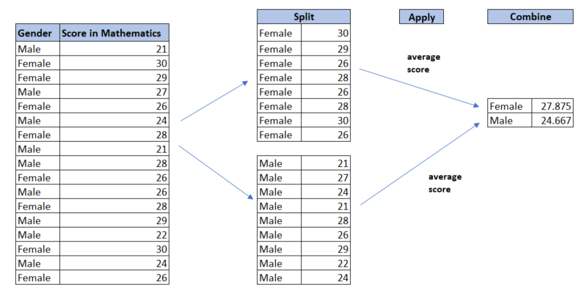
5.7.8 group_by() – Working with Groups

On its own, the group_by() function doesn’t perform any operation. However, when combined with functions like summarise() or mutate(), it becomes a powerful tool for splitting data into groups and applying operations to each group separately.

Key Points:

• Groups can be based on one or multiple variables.

• After grouping, any operation is applied independently to each group.

• The results are combined into a single data frame.

Figure 5.5 below illustrates the group by strategy:

Figure 5.5: Data Aggregation and Group Operations

Example 2: Summarising by Groups

To generate summaries for specific groups, combine summarise() with group_by():

msleep |>
  group_by(order) |>
  summarise(
    n = n(),
    average_sleep = mean(sleep_total, na.rm = TRUE),
    maximum_sleep = max(sleep_total, na.rm = TRUE)
  )

#> # A tibble: 19 × 4
#>    order               n average_sleep maximum_sleep
#>    <chr>           <int>         <dbl>         <dbl>
#>  1 Afrosoricida        1         15.6           15.6
#>  2 Artiodactyla        6          4.52           9.1
#>  3 Carnivora          12         10.1           15.8
#>  4 Cetacea             3          4.5            5.6
#>  5 Chiroptera          2         19.8           19.9
#>  6 Cingulata           2         17.8           18.1
#>  7 Didelphimorphia     2         18.7           19.4
#>  8 Diprotodontia       2         12.4           13.7
#>  9 Erinaceomorpha      2         10.2           10.3
#> 10 Hyracoidea          3          5.67           6.3
#> 11 Lagomorpha          1          8.4            8.4
#> 12 Monotremata         1          8.6            8.6
#> 13 Perissodactyla      3          3.47           4.4
#> 14 Pilosa              1         14.4           14.4
#> 15 Primates           12         10.5           17  
#> 16 Proboscidea         2          3.6            3.9
#> 17 Rodentia           22         12.5           16.6
#> 18 Scandentia          1          8.9            8.9
#> 19 Soricomorpha        5         11.1           14.9

Note

In this example:

• n: Number of species in each group.

• average_sleep: Average sleep time for each group, ignoring NA values (na.rm = TRUE).

• maximum_sleep: Maximum sleep time for each group, ignoring NA values.

Using summarise() with or without group_by() helps you aggregate and summarize your data efficiently, making it easier to extract meaningful insights from your dataset.

5.7.9 Combining All the Verbs:

Let’s tackle a realistic problem by chaining the verbs you’ve learned together. For this example, we’ll use the penguins dataset (from the palmerpenguins package) to answer a specific question:

Task:

Identify the top 5 penguins on Dream Island with flipper lengths exceeding 200 mm. Calculate their bill aspect ratio (bill length ÷ bill depth) and display the results sorted by this ratio.

# Load the dataset
penguins <- palmerpenguins::penguins

# Perform the analysis
penguins |>
  filter(island == "Dream" & flipper_length_mm > 200) |>
  mutate(bill_aspect_ratio = bill_length_mm / bill_depth_mm) |>
  slice_max(bill_aspect_ratio, n = 5) |>
  select(species, flipper_length_mm, bill_aspect_ratio)

#> # A tibble: 5 × 3
#>   species   flipper_length_mm bill_aspect_ratio
#>   <fct>                 <int>             <dbl>
#> 1 Chinstrap               201              2.87
#> 2 Chinstrap               207              2.82
#> 3 Chinstrap               201              2.75
#> 4 Chinstrap               203              2.71
#> 5 Chinstrap               201              2.71

Tip

This code performs the following steps:

1. Filter: Retains only penguins located on Dream Island with a flipper length greater than 200 mm.

2. Mutate: Calculates the bill_aspect_ratio by dividing bill_length_mm by bill_depth_mm.

3. Slice Max: Selects the top 5 penguins with the highest bill aspect ratios.

4. Select: Displays only the columns for species, flipper length, and bill aspect ratio.

5.7.10 Exercise 5.2.1: Top 5 Carnivorous Animals

Now, let’s extend your skills with a new challenge. Using the msleep dataset, identify the top 5 carnivorous animals that sleep the most and calculate their sleep-to-weight ratio to understand how sleep duration scales with body size.

Task: Complete the following code by replacing the placeholders (...) with the correct values:

msleep |>
  filter(vore == ...) |>
  mutate(sleep_to_weight = ... / ...) |>
  select(name, sleep_total, sleep_to_weight) |> 
  slice_max(sleep_total, n = ---)

Instructions

1. Replace ... with the appropriate filtering criteria and calculations.

2. Ensure the final code filters for carnivores, calculates the sleep_to-weight ratio, and returns the top 5 animals that sleep the most.

See the Solution to Exercise 5.2.1

5.7.11 Exploring More Functions in dplyr

The dplyr package offers a wealth of functions to simplify data manipulation, enabling you to efficiently clean, transform, and analyze data. In addition to the core verbs (filter(), select(), mutate(), arrange(), summarize()), there are other incredibly useful functions such as:

1. rename(): Rename columns in your dataset.

2. distinct(): Extract unique rows or values.

3. count(): Count occurrences of unique values in a variable.

4. relocate(): Reorder or reposition columns for better organization.

Table 5.2: Summary of other Functions in dplyr

Function	Purpose	Example Usage
rename()	Rename columns to more meaningful names	rename(new_name = old_name)
distinct()	Find unique rows or specific values	distinct(column1, column2)
count()	Count the frequency of unique values	count(column_name)
relocate()	Reorder columns for better organization	relocate(column_name, .before = another_column)

Let’s explore each of the functions in Table 5.2 in detail using the msleep dataset from ggplot2 and the penguins dataset from palmerpenguins.

5.7.11.1 rename() – Renaming Columns

The rename() function allows you to change column names to make them more meaningful or easier to work with. This is especially helpful when dealing with datasets that have poorly named columns.

Key Points:

• Syntax: rename(new_name = old_name)
• You can rename one or multiple columns at a time.
• The rest of the dataset remains unchanged.

Example 1: Renaming Columns in msleep

Rename the column name to animal_name and sleep_total to total_sleep:

msleep |>
  rename(
    animal_name = name,
    total_sleep = sleep_total
  )

#> # A tibble: 83 × 11
#>    animal_name  genus vore  order conservation total_sleep sleep_rem sleep_cycle
#>    <chr>        <chr> <chr> <chr> <chr>              <dbl>     <dbl>       <dbl>
#>  1 Cheetah      Acin… carni Carn… lc                  12.1      NA        NA    
#>  2 Owl monkey   Aotus omni  Prim… <NA>                17         1.8      NA    
#>  3 Mountain be… Aplo… herbi Rode… nt                  14.4       2.4      NA    
#>  4 Greater sho… Blar… omni  Sori… lc                  14.9       2.3       0.133
#>  5 Cow          Bos   herbi Arti… domesticated         4         0.7       0.667
#>  6 Three-toed … Brad… herbi Pilo… <NA>                14.4       2.2       0.767
#>  7 Northern fu… Call… carni Carn… vu                   8.7       1.4       0.383
#>  8 Vesper mouse Calo… <NA>  Rode… <NA>                 7        NA        NA    
#>  9 Dog          Canis carni Carn… domesticated        10.1       2.9       0.333
#> 10 Roe deer     Capr… herbi Arti… lc                   3        NA        NA    
#> # ℹ 73 more rows
#> # ℹ 3 more variables: awake <dbl>, brainwt <dbl>, bodywt <dbl>

Note

1. rename(animal_name = name) renames the name column to animal_name.
2. rename(total_sleep = sleep_total) renames sleep_total to total_sleep.
3. You can use this to make column names more descriptive.

Example 2:

Rename bill_length_mm to bill_length and flipper_length_mm to flipper_length in the penguins data:

penguins |>
  rename(
    bill_length = bill_length_mm,
    flipper_length = flipper_length_mm
  )

#> # A tibble: 344 × 8
#>    species island    bill_length bill_depth_mm flipper_length body_mass_g sex   
#>    <fct>   <fct>           <dbl>         <dbl>          <int>       <int> <fct> 
#>  1 Adelie  Torgersen        39.1          18.7            181        3750 male  
#>  2 Adelie  Torgersen        39.5          17.4            186        3800 female
#>  3 Adelie  Torgersen        40.3          18              195        3250 female
#>  4 Adelie  Torgersen        NA            NA               NA          NA <NA>  
#>  5 Adelie  Torgersen        36.7          19.3            193        3450 female
#>  6 Adelie  Torgersen        39.3          20.6            190        3650 male  
#>  7 Adelie  Torgersen        38.9          17.8            181        3625 female
#>  8 Adelie  Torgersen        39.2          19.6            195        4675 male  
#>  9 Adelie  Torgersen        34.1          18.1            193        3475 <NA>  
#> 10 Adelie  Torgersen        42            20.2            190        4250 <NA>  
#> # ℹ 334 more rows
#> # ℹ 1 more variable: year <int>

Reflection Question

How might renaming confusing column names or removing duplicates before analysis contribute to more confident and accurate inferences?

5.7.11.2 distinct() – Extracting Unique Rows or Values

Duplicates in datasets can distort analyses and lead to inaccurate conclusions. Identifying and removing duplicates ensures clean data that accurately represents unique observations. The distinct() function is a simple yet powerful tool for finding unique rows or specific combinations of values in a dataset. It is particularly useful for removing duplicate rows or understanding unique categories in a variable.

Key Points:

1. Default Behavior:
   By default, distinct() considers all columns to identify unique rows.

2. Specific Variables:
   You can specify one or more columns to extract unique values for specific variables.

3. Keeping All Variables:
   Adding .keep_all = TRUE while specifying columns ensures that all other variables are retained in the resulting dataset.

4. Using janitor::get_dupes():
   The get_dupes() function from the janitor package provides an easy way to identify duplicates. It returns:

   • Full records where the specified variables have duplicates.

   • A column called dupe_count showing the number of rows sharing each duplicate combination.

Example 1: Counting Duplicates (iris Dataset)

To count the number of duplicate rows in a dataset, use the combination of duplicated() and sum() functions:

sum(duplicated(iris))

#> [1] 1

There is one duplicate record found in this dataset.

Example 2: Identifying and Removing Duplicates (iris Dataset)

To find duplicate records in the iris dataset

iris |> janitor::get_dupes()

#> No variable names specified - using all columns.

#> # A tibble: 2 × 6
#>   Sepal.Length Sepal.Width Petal.Length Petal.Width Species   dupe_count
#>          <dbl>       <dbl>        <dbl>       <dbl> <fct>          <int>
#> 1          5.8         2.7          5.1         1.9 virginica          2
#> 2          5.8         2.7          5.1         1.9 virginica          2

The output shows the duplicate records in the iris dataset. To remove these duplicates and retain only the unique rows, you can use the distinct() function as follows:

iris |> distinct()

#> # A tibble: 149 × 5
#>    Sepal.Length Sepal.Width Petal.Length Petal.Width Species
#>           <dbl>       <dbl>        <dbl>       <dbl> <fct>  
#>  1          5.1         3.5          1.4         0.2 setosa 
#>  2          4.9         3            1.4         0.2 setosa 
#>  3          4.7         3.2          1.3         0.2 setosa 
#>  4          4.6         3.1          1.5         0.2 setosa 
#>  5          5           3.6          1.4         0.2 setosa 
#>  6          5.4         3.9          1.7         0.4 setosa 
#>  7          4.6         3.4          1.4         0.3 setosa 
#>  8          5           3.4          1.5         0.2 setosa 
#>  9          4.4         2.9          1.4         0.2 setosa 
#> 10          4.9         3.1          1.5         0.1 setosa 
#> # ℹ 139 more rows

Example 3: Finding Unique Values in a Specific Column (msleep Dataset)

To extract unique values from the vore column in the msleep dataset (diet types):

msleep |>
  distinct(vore)

#> # A tibble: 5 × 1
#>   vore   
#>   <chr>  
#> 1 carni  
#> 2 omni   
#> 3 herbi  
#> 4 <NA>   
#> 5 insecti

Note

The distinct(vore) function returns only the unique values in the vore column, helping you understand the categories in this variable.

Example 4: Keeping All Variables When Filtering for Uniqueness

To return unique rows based on the vore column while keeping all other variables:

msleep |>
  distinct(vore, .keep_all = TRUE)

#> # A tibble: 5 × 11
#>   name    genus vore  order conservation sleep_total sleep_rem sleep_cycle awake
#>   <chr>   <chr> <chr> <chr> <chr>              <dbl>     <dbl>       <dbl> <dbl>
#> 1 Cheetah Acin… carni Carn… lc                  12.1      NA        NA      11.9
#> 2 Owl mo… Aotus omni  Prim… <NA>                17         1.8      NA       7  
#> 3 Mounta… Aplo… herbi Rode… nt                  14.4       2.4      NA       9.6
#> 4 Vesper… Calo… <NA>  Rode… <NA>                 7        NA        NA      17  
#> 5 Big br… Epte… inse… Chir… lc                  19.7       3.9       0.117   4.3
#> # ℹ 2 more variables: brainwt <dbl>, bodywt <dbl>

Note

Adding .keep_all = TRUE ensures that the uniqueness is determined by the vore column, but all other columns are retained in the output.

5.7.11.3 count() – Counting Occurrences

The count() function is a quick way to calculate the frequency of unique values in a column or combinations of columns. It is particularly useful for summarizing categorical variables.

Adding the sort = TRUE argument will automatically sort the results in descending order of frequency.

Key Points:

• By default, count() returns the number of occurrences for each unique value.
• Use count(x, sort = TRUE) to sort the results, with the largest groups appearing at the top.

Example 1

Count the number of animals in each diet category (vore) in the msleep data:

msleep |>
  count(vore, sort = TRUE)

#> # A tibble: 5 × 2
#>   vore        n
#>   <chr>   <int>
#> 1 herbi      32
#> 2 omni       20
#> 3 carni      19
#> 4 <NA>        7
#> 5 insecti     5

Explanation:

1. count(vore) calculates how many times each diet type (vore) appears.

2. The output has two columns: vore and n (the count).

Example 2

Count the number of penguins on each island in the penguins data:

penguins |>
  count(island)

#> # A tibble: 3 × 2
#>   island        n
#>   <fct>     <int>
#> 1 Biscoe      168
#> 2 Dream       124
#> 3 Torgersen    52

5.7.11.4 relocate() – Reordering Columns

The relocate() function allows you to rearrange columns for better readability or logical grouping using the same syntax as select() to make it easy to move blocks of columns at once. It doesn’t remove or modify columns, only changes their position.

Key Points:

• Use relocate(column_name, .before = ...) to move a column before a specific column.

• Use relocate(column_name, .after = ...) to move a column after a specific column.

Example 1 : Reordering Columns in msleep

Move bodywt to appear after the sleep_total column:

msleep |>
  relocate(bodywt, .after = sleep_total)

#> # A tibble: 83 × 11
#>    name             genus vore  order conservation sleep_total  bodywt sleep_rem
#>    <chr>            <chr> <chr> <chr> <chr>              <dbl>   <dbl>     <dbl>
#>  1 Cheetah          Acin… carni Carn… lc                  12.1  50          NA  
#>  2 Owl monkey       Aotus omni  Prim… <NA>                17     0.48        1.8
#>  3 Mountain beaver  Aplo… herbi Rode… nt                  14.4   1.35        2.4
#>  4 Greater short-t… Blar… omni  Sori… lc                  14.9   0.019       2.3
#>  5 Cow              Bos   herbi Arti… domesticated         4   600           0.7
#>  6 Three-toed sloth Brad… herbi Pilo… <NA>                14.4   3.85        2.2
#>  7 Northern fur se… Call… carni Carn… vu                   8.7  20.5         1.4
#>  8 Vesper mouse     Calo… <NA>  Rode… <NA>                 7     0.045      NA  
#>  9 Dog              Canis carni Carn… domesticated        10.1  14           2.9
#> 10 Roe deer         Capr… herbi Arti… lc                   3    14.8        NA  
#> # ℹ 73 more rows
#> # ℹ 3 more variables: sleep_cycle <dbl>, awake <dbl>, brainwt <dbl>

Example 2:

You can also relocate variables based on their data type:

penguins |> relocate(where(is.factor), .before = bill_length_mm)

#> # A tibble: 344 × 8
#>    species island    sex    bill_length_mm bill_depth_mm flipper_length_mm
#>    <fct>   <fct>     <fct>           <dbl>         <dbl>             <int>
#>  1 Adelie  Torgersen male             39.1          18.7               181
#>  2 Adelie  Torgersen female           39.5          17.4               186
#>  3 Adelie  Torgersen female           40.3          18                 195
#>  4 Adelie  Torgersen <NA>             NA            NA                  NA
#>  5 Adelie  Torgersen female           36.7          19.3               193
#>  6 Adelie  Torgersen male             39.3          20.6               190
#>  7 Adelie  Torgersen female           38.9          17.8               181
#>  8 Adelie  Torgersen male             39.2          19.6               195
#>  9 Adelie  Torgersen <NA>             34.1          18.1               193
#> 10 Adelie  Torgersen <NA>             42            20.2               190
#> # ℹ 334 more rows
#> # ℹ 2 more variables: body_mass_g <int>, year <int>

Combining These Functions

Let’s combine rename(), distinct(), count(), and relocate() to solve a real-world problem.

Example: Cleaning and Organizing msleep Data

1. Rename columns for clarity.

2. Remove duplicate rows.

3. Reorganize columns for better readability.

4. Count occurrences of diet types.

msleep |>
  rename(
    animal_name = name,
    diet_type = vore
  ) |>
  distinct() |>
  relocate(diet_type, .before = animal_name) |>
  count(diet_type, sort = TRUE)

#> # A tibble: 5 × 2
#>   diet_type     n
#>   <chr>     <int>
#> 1 herbi        32
#> 2 omni         20
#> 3 carni        19
#> 4 <NA>          7
#> 5 insecti       5

5.7.12 Practice Quiz 5.2

Question 1:

Which function would you use in dplyr to randomly select a specified number of rows from a dataset?

1. sample(n = 5)
   
2. slice_sample(n = 5)
   
3. filter_sample()
   
4. mutate_sample()

Question 2:

To calculate the average sleep_total for each vore category, which combination of functions is most appropriate?

1. group_by(vore) |> select(sleep_total) |> summarise(mean(sleep_total))

2. select(vore, sleep_total) |> summarise(mean(sleep_total)) |> group_by(vore)

3. group_by(vore) |> summarise(avg_sleep = mean(sleep_total, na.rm = TRUE))

4. filter(vore) |> mutate(avg_sleep = mean(sleep_total))

Question 3:

To extract rows with the maximum value of a specified variable, which function is appropriate in dplyr?

1. slice_max()
   
2. slice_min()
   
3. mutate()
   
4. select()

Question 4:

Which dplyr function would you use if you want to create a new column called weight_ratio by dividing bodywt by mean_bodywt?

1. filter()
   
2. select()
   
3. mutate()
   
4. arrange()

Question 5:

Suppose you need to identify the top 3 penguins with the highest bill aspect ratio from the penguins dataset after calculating it in a new column. Which of the following code snippets is the most concise and appropriate?

penguins |>
  mutate(bill_aspect_ratio = bill_length_mm / bill_depth_mm) |>
  arrange(desc(bill_aspect_ratio)) |>
  head(3)

penguins |>
  mutate(bill_aspect_ratio = bill_length_mm / bill_depth_mm) |>
  slice_max(bill_aspect_ratio, n = 3)

3. Both a and b are equally concise and valid.

4. Neither a nor b is valid.

Question 6:

Given the following code, which is the correct equivalent using the pipe operator?

result <- arrange(filter(select(msleep, name, sleep_total), sleep_total > 8), sleep_total)

1. msleep |> select(name, sleep_total) |> filter(sleep_total > 8) |> arrange(sleep_total)
   

2. msleep |> filter(sleep_total > 8) |> select(name, sleep_total) |> arrange(sleep_total)

3. select(msleep, name, sleep_total) |> filter(sleep_total > 8) |> arrange(sleep_total)

4. msleep |> arrange(sleep_total) |> filter(sleep_total > 8) |> select(name, sleep_total)

Question 7:

Which of the following correctly applies a log transformation to numeric columns only?

mutate_all(log)

mutate(across(everything(), log))

mutate(select(where(is.numeric), log))

mutate(across(where(is.numeric), log))

Question 8:

What does mutate(across(everything(), as.character)) do?

1. Converts all character columns to numeric.
   
2. Converts all columns in the dataset to character type.
   
3. Applies a conditional transformation to numeric columns.
   
4. Filters out non-character values.

Question 9:

To extract the rows with the minimum value of a specified variable, which dplyr function should you use?

1. slice_min()
   
2. slice_max()
   
3. arrange()
   
4. filter()

Question 10:

If you want to reorder the rows of msleep by sleep_total in ascending order and then only show the top 5 rows, which code snippet is correct?

1. msleep |> arrange(sleep_total) |> head(5)

2. msleep |> head(5) |> arrange(sleep_total)

3. msleep |> summarise(sleep_total) |> head(5)
   

4. msleep |> select(sleep_total) |> arrange(desc(sleep_total)) |> head(5)

See the Solution to Quiz 5.2

5.7.13 Exercise 5.2.2: Analysing the Penguins Dataset

Let’s put your skills into practice with a modified penguins dataset. First, you’ll need to create a new RStudio project called Experiment 5.1.

1. Importing and Inspecting Data

   • Locate the penguins.xlsx file in the r-data directory. If you don’t already have the file, you can download it from Google Drive.

   • Import the data into R.

   • Use glimpse(penguins) to get an overview.

   • How many rows and columns are there?

2. Filtering Data

   • How many penguins are from the Biscoe island?

   • Extract data for penguins with a body mass greater than 4,500 grams.

3. Arranging Data

   • Arrange the data in descending order based on flipper length.

   • Find the top 5 penguins with the highest body mass.

4. Selecting and Mutating

   • Select only the columns species, island, and sex.

   • Remove the sex column from the dataset.

   • Convert the flipper length from millimeters to meters and create a new column flipper_length_m

     To convert millimeters to meters, you simply divide the number of millimeters by 1,000. Here’s the conversion formula:

     \[\text{flipper\_length\_m} = \frac{\text{flipper\_length\_mm}}{1000}\]

   • Create a new column BMI calculated as:

     \[\text{BMI} = \frac{\text{body\_mass\_g}}{{\text{flipper\_length\_m}}^2}\]

5. Summarizing and Grouping

   • Calculate the average body mass of all penguins.

   • Group the data by species and find the average body mass for each species.

6. Combining Operations

   • Filter penguins from the Dream island and summarize the average bill length for each species from this island.

5.7.14 Exercise 5.2.3: Data Analyst Candidate Assessment

In this exercise, you’ll work with a real dataset of medical insurance records similar to those of a well-known health insurance company in the country. We want to see how you clean, transform and analyse data in a practical, real-world context as a Data Analyst. Please follow the instructions below and document your process along the way.

Dataset Overview

You’re provided with a dataset containing medical insurance records for various individuals. Here’s what each column represents:

• User ID: A unique identifier for each individual.

• Gender: The individual’s gender (‘Male’ or ‘Female’).

• Age: The age of the individual in years.

• AgeGroup: The age bracket into which the individual falls.

• Estimated Salary: An estimate of the individual’s annual salary.

• Purchased: Indicates whether the individual has purchased medical insurance (‘purchased’ or ‘not-purchased’).

Data Import Instructions

1. Locate the medical_insurance.xlsx file in the r-data directory. If you don’t have it yet, you can download it from Google Drive.

2. Import the dataset into R using the readxl package.

Tasks

1. Data Transformation

• Purchased Column Conversion:
  Convert the Purchased column values to binary: use 1 for ‘purchased’ and 0 for ‘not-purchased’.

• Creating Salary Brackets:
  Add a new column called SalaryBracket based on the Estimated Salary:

  • Low: Salary < 30,000
    
  • Medium: Salary between 30,000 and 70,000
    
  • High: Salary > 70,000

2. Analysis and Insights

• Insurance Purchase Analysis:
  Calculate and present:

  • The percentage of individuals who have purchased insurance, broken down by Gender.
  • The percentage of individuals who have purchased insurance, broken down by AgeGroup.

• Salary Bracket Purchase Rate:
  Determine which SalaryBracket shows the highest rate of insurance purchases.

Note

Take your time to work through these tasks carefully. We’re looking forward to seeing how you apply your analytical skills to solve real-world data challenges. Good luck!

5.8 Experiment 5.3: Dealing with Missing Data

Missing data is common in real-world scenarios. Values may be missing because of measurement errors, data entry mistakes, or unavailability of certain information. It is crucial to detect and handle missing values properly, as they can bias results or cause errors in your analysis. R provides several functions to help you deal with missing data.

5.8.1 Recognising Missing Values

In R, missing values are represented by NA. Identifying these missing values is crucial for accurate data analysis. Here are some functions to check for missing data:

• is.na(): Returns a logical vector indicating which elements are NA.

  x <- c(1, 2, NA, 4, NA, 6)
  
  is.na(x)

  #> [1] FALSE FALSE  TRUE FALSE  TRUE FALSE

• anyNA(): Checks if there are any NA values in an object. It returns TRUE if there is at least one NA, and FALSE otherwise.

  anyNA(x)

  #> [1] TRUE

Let’s apply the anyNA() function to a sample salary_data data frame:

salary_data <- data.frame(
  Name = c("Alice", "Francisca", "Fatima", "David"),
  Age = c(25, NA, 30, 35),
  Salary = c(50000, 52000, NA, 55000)
)

salary_data

#>        Name Age Salary
#> 1     Alice  25  50000
#> 2 Francisca  NA  52000
#> 3    Fatima  30     NA
#> 4     David  35  55000

In this data frame, Francisca’s age and Fatima’s salary are missing. We can use anyNA() to check whether there are any missing values in the entire data frame:

anyNA(salary_data)

#> [1] TRUE

Since the output is TRUE, we know there are missing values. We can also check specific columns for missing values. For example, let’s check the Age column:

anyNA(salary_data$Age)

#> [1] TRUE

And similarly, we can check the Name column:

anyNA(salary_data$Name)

#> [1] FALSE

• complete.cases(): Identifies rows in a dataset that have no missing values (NA). It evaluates each row and checks whether it is “complete” (i.e., contains no NA values). It returns a logical vector where:

  • TRUE indicates that a row has no missing values (all columns are complete).

  • FALSE indicates that a row contains at least one missing value.

For example, using our sample salary_data data frame:

salary_data

#>        Name Age Salary
#> 1     Alice  25  50000
#> 2 Francisca  NA  52000
#> 3    Fatima  30     NA
#> 4     David  35  55000

complete.cases(salary_data)

#> [1]  TRUE FALSE FALSE  TRUE

Note

This indicates that:

• Row 1 (Alice): No missing values, so it is complete (TRUE).

• Row 2 (Francisca): Missing value in the Age column, so it is not complete (FALSE).

• Row 3 (Fatima): Missing value in the Salary column, so it is not complete (FALSE).

• Row 4 (David): No missing values, so it is complete (TRUE).

5.8.2 Summarising Missing Data

After identifying that your dataset contains missing values, it’s essential to quantify them to understand the extent of the issue. Summarizing missing data helps you decide how to handle these gaps appropriately. To count the total number of missing values in your entire dataset, you can use the sum() function combined with is.na(). Remember the is.na() function returns a logical vector where each element is TRUE if the corresponding value in the dataset is NA, and FALSE otherwise. Summing this logical vector gives you the total count of missing values because TRUE is treated as 1 and FALSE as 0 in arithmetic operations.

Example:

Suppose you have a sampled airquality dataset:

airquality_data <- data.frame(
  Ozone = c(41, 36, 12, 18, NA, 28, 23, 19, 8, NA),
  Solar.R = c(190, 118, 149, 313, NA, NA, 299, 99, 19, 194),
  Wind = c(7.4, 8, 12.6, 11.5, 14.3, 14.9, 8.6, 13.8, 20.1, 8.6),
  Temp = c(67, 72, 74, 62, 56, 66, 65, 59, 61, 69),
  Month = c(5, 5, 5, NA, NA, NA, 5, 5, 5, 5),
  Day = c(1, 2, 3, 4, 5, 6, 7, 8, 9, 10)
)

airquality_data

#>    Ozone Solar.R Wind Temp Month Day
#> 1     41     190  7.4   67     5   1
#> 2     36     118  8.0   72     5   2
#> 3     12     149 12.6   74     5   3
#> 4     18     313 11.5   62    NA   4
#> 5     NA      NA 14.3   56    NA   5
#> 6     28      NA 14.9   66    NA   6
#> 7     23     299  8.6   65     5   7
#> 8     19      99 13.8   59     5   8
#> 9      8      19 20.1   61     5   9
#> 10    NA     194  8.6   69     5  10

To count the total number of missing values in this dataset, you would use:

sum(is.na(airquality_data))

#> [1] 7

There are 7 missing values in the entire data frame.

Missing Values Per Column:

colSums(is.na(airquality_data))

#>   Ozone Solar.R    Wind    Temp   Month     Day 
#>       2       2       0       0       3       0

This output indicates:

• Ozone column has 2 missing values.

• Solar.R column has 2 missing values.

• Wind column has 0 missing values.

• Temp column has 0 missing values.

• Month column has 3 missing values.

• Daycolumn has 0 missing values.

For a column-wise summary, you can also use the inspect_na() function from the inspectdf package.

inspectdf::inspect_na(airquality_data)

#> # A tibble: 6 × 3
#>   col_name   cnt  pcnt
#>   <chr>    <int> <dbl>
#> 1 Month        3    30
#> 2 Ozone        2    20
#> 3 Solar.R      2    20
#> 4 Wind         0     0
#> 5 Temp         0     0
#> 6 Day          0     0

5.8.3 Strategies for Dealing with Missing Data

Managing missing data is a critical step in data preprocessing. There are several strategies available, depending on the nature of the data and the goals of the analysis.

5.8.3.1 Remove Missing Values

You can remove rows with missing values using na.omit() function:

cleaned_data <- na.omit(airquality_data)
cleaned_data

#>   Ozone Solar.R Wind Temp Month Day
#> 1    41     190  7.4   67     5   1
#> 2    36     118  8.0   72     5   2
#> 3    12     149 12.6   74     5   3
#> 7    23     299  8.6   65     5   7
#> 8    19      99 13.8   59     5   8
#> 9     8      19 20.1   61     5   9

Warning

This method is simple and effective when the proportion of missing data is small. However, it can result in a significant loss of data if many rows contain missing values.

5.8.3.2 Replace Missing Values

Replace missing values with a default value using replace_na() from the tidyr package:

library(tidyverse) # tidyr is part of tidyverse
dataset <- airquality_data %>%
  replace_na(list(Ozone = 17, Month = 3))

dataset

#>    Ozone Solar.R Wind Temp Month Day
#> 1     41     190  7.4   67     5   1
#> 2     36     118  8.0   72     5   2
#> 3     12     149 12.6   74     5   3
#> 4     18     313 11.5   62     3   4
#> 5     17      NA 14.3   56     3   5
#> 6     28      NA 14.9   66     3   6
#> 7     23     299  8.6   65     5   7
#> 8     19      99 13.8   59     5   8
#> 9      8      19 20.1   61     5   9
#> 10    17     194  8.6   69     5  10

Note

This approach ensures that missing values are replaced consistently, allowing for meaningful analysis without introducing bias.

5.8.3.3 Impute Missing Values

Missing values can be replaced with statistical measures such as the mean, median, or mode. For example, missing values in the Ozone column can be replaced with the mean, while missing values in the Month column can be replaced with the median:

library(dplyr)

airquality_data <- airquality_data %>%
  mutate(
    Ozone = ifelse(is.na(Ozone), mean(Ozone, na.rm = TRUE), Ozone),
    Month = ifelse(is.na(Month), median(Month, na.rm = TRUE), Month)
  )

# View the resulting dataset
airquality_data

#>     Ozone Solar.R Wind Temp Month Day
#> 1  41.000     190  7.4   67     5   1
#> 2  36.000     118  8.0   72     5   2
#> 3  12.000     149 12.6   74     5   3
#> 4  18.000     313 11.5   62     5   4
#> 5  23.125      NA 14.3   56     5   5
#> 6  28.000      NA 14.9   66     5   6
#> 7  23.000     299  8.6   65     5   7
#> 8  19.000      99 13.8   59     5   8
#> 9   8.000      19 20.1   61     5   9
#> 10 23.125     194  8.6   69     5  10

Tip

If you don’t want to use ifelse, you can achieve the same result using the coalesce() function from dplyr. coalesce() replaces NA values by providing a fallback value.

library(dplyr)

airquality_data <- airquality_data %>%
  mutate(
    Ozone = coalesce(Ozone, mean(Ozone, na.rm = TRUE)),
    Month = coalesce(Month, median(Month, na.rm = TRUE))
  )

# View the resulting dataset
airquality_data

#>     Ozone Solar.R Wind Temp Month Day
#> 1  41.000     190  7.4   67     5   1
#> 2  36.000     118  8.0   72     5   2
#> 3  12.000     149 12.6   74     5   3
#> 4  18.000     313 11.5   62     5   4
#> 5  23.125      NA 14.3   56     5   5
#> 6  28.000      NA 14.9   66     5   6
#> 7  23.000     299  8.6   65     5   7
#> 8  19.000      99 13.8   59     5   8
#> 9   8.000      19 20.1   61     5   9
#> 10 23.125     194  8.6   69     5  10

• coalesce() is a simpler and more concise alternative when dealing with missing values.

• coalesce(Ozone, mean(Ozone, na.rm = TRUE)) replaces NA values in Ozone with the computed mean.

• coalesce(Month, median(Month, na.rm = TRUE)) does the same for Month using the median.

For more advanced imputation methods, you can use specialised packages like mice or Hmisc. Additionally, the bulkreadr package simplifies the process with the fill_missing_values() function:

• Impute Specific Columns:

  library(bulkreadr)
  
  fill_missing_values(airquality_data,
    selected_variables = c("Ozone", "Solar.R"),
    method = "mean"
  )

  #>     Ozone Solar.R Wind Temp Month Day
  #> 1  41.000 190.000  7.4   67     5   1
  #> 2  36.000 118.000  8.0   72     5   2
  #> 3  12.000 149.000 12.6   74     5   3
  #> 4  18.000 313.000 11.5   62     5   4
  #> 5  23.125 172.625 14.3   56     5   5
  #> 6  28.000 172.625 14.9   66     5   6
  #> 7  23.000 299.000  8.6   65     5   7
  #> 8  19.000  99.000 13.8   59     5   8
  #> 9   8.000  19.000 20.1   61     5   9
  #> 10 23.125 194.000  8.6   69     5  10

• Impute All Columns in the Data Frame:

  fill_missing_values(airquality_data, method = "median")

  #>     Ozone Solar.R Wind Temp Month Day
  #> 1  41.000   190.0  7.4   67     5   1
  #> 2  36.000   118.0  8.0   72     5   2
  #> 3  12.000   149.0 12.6   74     5   3
  #> 4  18.000   313.0 11.5   62     5   4
  #> 5  23.125   169.5 14.3   56     5   5
  #> 6  28.000   169.5 14.9   66     5   6
  #> 7  23.000   299.0  8.6   65     5   7
  #> 8  19.000    99.0 13.8   59     5   8
  #> 9   8.000    19.0 20.1   61     5   9
  #> 10 23.125   194.0  8.6   69     5  10

Warning

This approach helps to preserve the structure of the dataset and minimises data loss. However, it can introduce bias if the chosen statistic (e.g., mean or median) does not accurately represent the underlying data.

5.8.3.4 Flag Missing Data

You can create a new column to flag rows with missing values:

airquality_data %>% mutate(missing_flag = !complete.cases(.))

#>     Ozone Solar.R Wind Temp Month Day missing_flag
#> 1  41.000     190  7.4   67     5   1        FALSE
#> 2  36.000     118  8.0   72     5   2        FALSE
#> 3  12.000     149 12.6   74     5   3        FALSE
#> 4  18.000     313 11.5   62     5   4        FALSE
#> 5  23.125      NA 14.3   56     5   5         TRUE
#> 6  28.000      NA 14.9   66     5   6         TRUE
#> 7  23.000     299  8.6   65     5   7        FALSE
#> 8  19.000      99 13.8   59     5   8        FALSE
#> 9   8.000      19 20.1   61     5   9        FALSE
#> 10 23.125     194  8.6   69     5  10        FALSE

Tip

Using !complete.cases(.) ensures the missing_flag column accurately identifies rows with missing values (TRUE) while marking rows without missing values as FALSE. This binary flag is useful for quickly filtering or inspecting incomplete data.

Alternatively, instead of a binary flag, you can add a column that shows the number of missing values in each row:

airquality_data$missing_count <- rowSums(is.na(airquality_data))

airquality_data

#>     Ozone Solar.R Wind Temp Month Day missing_count
#> 1  41.000     190  7.4   67     5   1             0
#> 2  36.000     118  8.0   72     5   2             0
#> 3  12.000     149 12.6   74     5   3             0
#> 4  18.000     313 11.5   62     5   4             0
#> 5  23.125      NA 14.3   56     5   5             1
#> 6  28.000      NA 14.9   66     5   6             1
#> 7  23.000     299  8.6   65     5   7             0
#> 8  19.000      99 13.8   59     5   8             0
#> 9   8.000      19 20.1   61     5   9             0
#> 10 23.125     194  8.6   69     5  10             0

Tip

Adding a column like missing_count provides a numeric indicator of the total number of missing values in each row. This approach is particularly helpful when you need to assess the extent of missingness across the dataset or prioritise rows for further investigation

Reflection Question

Consider the potential biases introduced by removing all rows with missing values. In which scenarios would you prefer imputation over removal?

5.8.4 Practice Quiz 5.3

Question 1:

Which function in R checks if there are any missing values in an object?

1. is.na()
   
2. anyNA()
   
3. complete.cases()
   
4. na.omit()

Question 2:

Which approach removes any rows containing NA values?

1. na.omit()
   
2. replace_na()
   
3. complete.cases()
   
4. anyNA()

Question 3:

If you decide to impute missing values in a column using the median, what is one potential advantage of using the median rather than the mean?

1. The median is always easier to compute.
   
2. The median is more affected by outliers than the mean.
   
3. The median is less influenced by extreme values and may provide a more robust estimate.
   
4. The median will always be exactly halfway between the min and max values.

Question 4:

How would you replace all NA values in character columns with "Unknown"?

mutate(across(where(is.character), ~ replace_na(., "Unknown")))

mutate_all(~ replace_na(., "Unknown"))

mutate(across(where(is.character), na.omit))

mutate(across(where(is.character), replace(. == NA, "Unknown")))

Question 5:

What does the anyNA() function return?

1. The number of missing values in an object.
   
2. TRUE if there are any missing values in the object; otherwise, FALSE.
   
3. A logical vector of missing values in each row.
   
4. A subset of the data frame without missing values.

Question 6:

You want to create a new column in a data frame that flags rows with missing values as TRUE. Which code achieves this?

1. df$new_col <- !complete.cases(df)
2. df$new_col <- complete.cases(df)
   
3. df$new_col <- anyNA(df)
   
4. df$new_col <- is.na(df)

Question 7:

Before removing rows with missing values, what is an important consideration?

1. Whether the missing values are randomly distributed across the data.
   
2. Whether the dataset is stored in a data frame.
   
3. Whether missing values exist in every column.
   
4. Whether the missing values are encoded as NA.

Question 8:

Why should the proportion of missing data in a row or column be considered before removing it?

1. Removing rows or columns with minimal missing values may lead to excessive data loss.
   
2. Columns with missing values cannot be visualized.
   
3. Rows with missing values are always irrelevant.
   
4. Rows with missing values should never be analyzed.

Question 9:

If a dataset has 50% missing values in a column, what is a common approach to handle this situation?

1. Replace missing values with the column mean.
   
2. Remove the column entirely.
   
3. Replace missing values with zeros.
   
4. Leave the missing values as they are.

Question 10:

What does the following Tidyverse-style code do?

library(dplyr)

airquality_data <- airquality_data %>%
  mutate(Ozone = if_else(is.na(Ozone), mean(Ozone, na.rm = TRUE), Ozone))

1. Removes rows where Ozone is missing.
   
2. Replaces missing values in Ozone with the mean of the column.
   
3. Flags rows where Ozone is missing.
   
4. Deletes the Ozone column if it has missing values.

See the Solution to Quiz 5.3

5.8.5 Exercise 5.3.1: Handling Missing Data in the Television Company Dataset

This exercise will test your data cleaning skills using the data-tv-company.csv dataset, located in the r-data directory. If you do not already have the file, you can download it from Google Drive.

Dataset Metadata

This dataset was collected by a small television company seeking to understand the factors that influence how viewers rate the company. It includes viewer ratings and related measures. The variables in the dataset are as follows:

• regard: Viewer rating of the television company (higher ratings indicate greater regard).

• gender: The gender with which the viewer identifies.

• views: The number of views.

• online: The number of times bonus online material was accessed.

• library: The number of times the online library was browsed.

• Show1 to Show4: Scores for four different shows.

Tasks

1. Importing and Inspecting Data

   • Locate the data-tv-company.csv file in the r-data directory.
   • Import the data into your R environment.
   • Inspect the dataset for any missing values.

2. Strategies for Dealing with Missing Data

   • Demonstrate at least four different methods for handling missing data in this dataset.
   • Apply these methods to the imported data.
   • Evaluate the methods and select the best approach based on your analysis.

See the Solution to Exercise 5.3.1

5.9 Reflective Summary

In Lab 5, you developed essential skills in data transformation with R, including::

• The Pipe Operator |>: You learned to link functions in a logical sequence, enhancing code readability.

• Data Manipulation with dplyr: You used core verbs—select(), filter(), mutate(), arrange(), and summarise()—to reshape and refine your data.

• Summarisation and Grouping: By using group_by() and summarise(), you aggregated data to uncover patterns and derive insights.

• Handling Missing Data: You learned to detect and manage missing values, ensuring the quality of your analysis.

These techniques form a crucial step in the data analysis pipeline, enabling you to approach complex datasets with confidence and produce meaningful insights.

What’s Next?

In the next lab, we will explore tidy data and joins. You will learn to reshape datasets and merge diverse data sources, converting raw data into structured, analysis-ready formats. This will pave the way for deeper insights and more efficient workflows.

---

1. The |> operator (called a pipe) means “and then.” It passes the result of one function to the next.

2. If you haven’t installed it yet, you can do so with install.packages("palmerpenguins") and load it using library(palmerpenguins).

3. Horst AM, Hill AP, Gorman KB (2020). palmerpenguins: Palmer Archipelago (Antarctica) penguin data. R package version 0.1.0. https://allisonhorst.github.io/palmerpenguins/. doi: 10.5281/zenodo.3960218.

4. Siegel, J. M. (2005). Clues to the functions of mammalian sleep. Nature, 437(7063), 1264-1271.

5. Using the same example, the syntax for across() with column positions would be as follows: msleep |> select(name, contains("sleep")) |> mutate(across(c(2, 3, 4), ~ .x * 60))

6. The between() function simplifies the code and improves readability by combining the range condition into a single statement.

7. While slice() selects rows based on their numeric position (e.g., the first or last few rows), without reordering the entire dataset, the arrange() function is used to reorder all rows in the dataset according to the values of one or more specified columns.