9  Sampling Techniques

9.1 Introduction

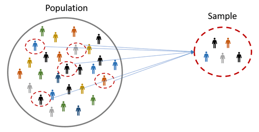
Welcome to Lab 9, where we will focus on understanding and applying sampling techniques. In the world of data analysis and statistics, drawing reliable conclusions often depends on how we collect our data. Since it’s rarely feasible—financially or logistically—to gather information from every member of a population, we turn to sampling. Sampling is the process of selecting a subset of individuals, observations, or objects from a larger population. If done properly, sampling allows us to save time, money, and effort while still gaining valuable insights that can accurately represent the entire group.

Figure 9.1: Population and Sample Illustration

Sampling is a cornerstone of research, and how you choose your sample can determine the accuracy and credibility of your conclusions. Consider the challenge of predicting election results: it would be impossible to survey every single voter. Instead, we carefully select a smaller group that reflects the overall population. By choosing the right sampling technique, we can make meaningful predictions and avoid misleading outcomes.

In this lab, we will explore both probability and non-probability sampling methods. You’ll learn about a range of techniques, their pros and cons, and the situations in which each method is most appropriate. We will also practice implementing these approaches in R, allowing you to reinforce these concepts with hands-on experience.

9.2 Learning Objectives

By the end of this lab, you should be able to:

• Understand Probability vs. Non-Probability Sampling:
  Recognize how probability sampling allows for generalizing results, while non-probability methods are often used for exploratory or hard-to-reach populations.

• Describe Common Probability Sampling Methods:
  Learn about simple random, stratified, cluster, and systematic sampling, and understand when to use each method.

• Describe Common Non-Probability Sampling Methods:
  Understand convenience, snowball, judgmental (purposive), and quota sampling, and appreciate their limitations.

• Match Methods to Research Scenarios:
  Identify which sampling strategy is most suitable given the research goals, data availability, and constraints.

• Reflect on Trade-Offs:
  Consider the strengths and weaknesses of different sampling approaches and how these choices affect your ability to generalize findings.

By completing this lab, you’ll be better equipped to design robust studies, interpret results confidently, and ensure that your data-driven conclusions stand on a solid methodological foundation.

9.3 Why Do We Sample?

Imagine you want to understand the average height of all adults in your country. Actually measuring every adult’s height would be incredibly difficult, time-consuming, and expensive. Instead, you might measure a carefully chosen group (sample) that fairly represents the entire population. From this sample, you can estimate the overall average height. But if your sample is biased or poorly chosen, your conclusions may be misleading. That’s why thoughtful sampling techniques matter.

9.4 Sampling Terminology

• Population: The entire group of individuals or items of interest.

• Sample: A subset of the population selected for analysis.

• Sampling Frame: A list or other resource that identifies all or most members of the population, from which we select the sample.

• Parameter: A numerical summary (e.g., mean, proportion) that describes some characteristic of the population.

• Statistic: A numerical summary that describes some characteristic of the sample, used to estimate the corresponding population parameter.

9.5 Understanding Probability and Non-Probability Sampling

In research, the strategies we use to select samples can vary greatly depending on the discipline, research area, and specific study. Broadly speaking, there are two main types of sampling methods: probability sampling and non-probability sampling.

Figure 9.2: Overview of Sampling Methods

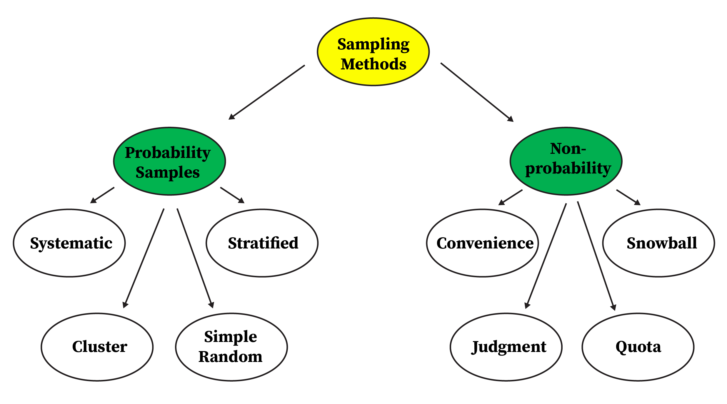
Probability Sampling

Probability Sampling methods ensure that every member of the population has a known chance of being included in the sample. This randomness allows you to measure how much uncertainty exists in your estimates. With probability sampling, statistical theory helps you gauge how closely your sample results match the real population values.

Non-Probability Sampling

Non-probability sampling methods do not rely on random selection; instead, they are based on subjective judgement, convenience, referrals, or other non-random criteria. Because not every member of the population necessarily has a known or equal chance of being included, these approaches often lack representativeness and make it harder to generalize results with confidence. Nevertheless, they are commonly used in exploratory research, when dealing with hidden populations, or under severe time and resource constraints, even though their inherent bias can complicate accuracy and limit the applicability of findings.

Reflection Question 1

Why might you choose a non-probability sampling method if it doesn’t allow you to confidently generalize findings to the entire population?

9.6 Experiment 9.1: Probability Sampling Techniques

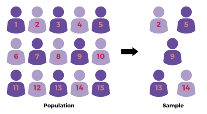
9.6.1 Simple Random Sampling (SRS)

In a simple random sample, every member of the population has an equal probability of being selected. This is often considered the “gold standard” because it tends to produce unbiased estimates if done correctly. It’s like pulling names out of a hat—no individual is favoured over another.

Figure 9.3: Simple Random Sampling Process

When to Use:

• When you have a well-defined population and a good sampling frame.

• When you want each unit in the population to have an equal chance of selection.

• When you do not need to target specific subgroups.

Pros:

Minimizes selection bias and is straightforward to implement if a complete list (sampling frame) exists.

Cons:

Can be difficult when the population is very large or when no complete sampling frame is available.

Example Scenario:

Suppose a university wants to know the average study time of its undergraduate students. Since the university has access to a complete list of all undergraduates, it can take a simple random sample of a few hundred students to estimate the overall average study time. Each student in the population would be equally likely to be selected, ensuring an unbiased estimate if done correctly.

Example Scenario using R:

Before coding, imagine having a large jar with 10,000 student IDs. To find out the average time they spend studying, you wouldn’t ask all 10,000 students—too time-consuming. Instead, you mix the IDs thoroughly and draw 500 at random, giving each student an equal chance of selection. In R, we’ll recreate this process by using a numeric vector of 10,000 IDs and randomly selecting 500 from it. This smaller group will help us reliably estimate the overall average study time. Here’s how:

# Ensures that we get the same random sample each time for reproducibility
set.seed(123)

# Imagine this is our complete list of undergraduates, each assigned a unique ID
student_ids <- 1:10000

# Draw a simple random sample of 500 students from the 10,000
sample_srs <- sample(student_ids, size = 500, replace = FALSE)

# Shows the first few sampled student IDs
head(sample_srs)

#> [1] 2463 2511 8718 2986 1842 9334

By running this code, you’ll see a handful of randomly chosen IDs. These represent your simple random sample—your mini version of the entire student body—ready for you to contact and measure their study hours.

9.6.2 Exercise 9.1.1: Simple Random Sampling with the Penguins Dataset

Use the penguins dataset from the palmerpenguins package to perform a simple random sample of 10 penguins. Compare the mean body mass of this sample to the mean body mass of the entire dataset.

Steps:

1. Load the palmerpenguins package and examine the penguins dataset.

2. Remove any rows with missing values to ensure you have a complete dataset.

3. Set a seed for reproducibility.

4. Select a simple random sample of 10 penguins from the complete dataset.

5. Calculate the mean body mass of the entire dataset.

6. Calculate the mean body mass of your sample.

7. Compare these two means and reflect on any differences.

See the Solution to Exercise 9.1.1

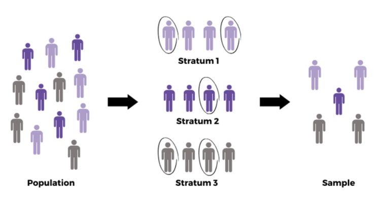
9.6.3 Stratified Sampling

Stratified sampling involves dividing the population into distinct subgroups (called strata) and then taking a proportional random sample from each subgroup. Strata are often formed based on characteristics you care about—like gender, age range, or region.

Figure 9.4: Stratified Sampling Process

When to Use:

• When the population is heterogeneous, and you want to ensure representation from all key subgroups.

• When you know something about how the population differs and you want your sample to reflect those differences accurately.

Pros:

Ensures that important subgroups are properly represented, leading to more precise estimates.

Cons:

Requires that you can clearly define and identify meaningful strata.

Example Scenario:

Suppose you want to survey residents of a country about their internet usage. You know age affects usage patterns, so you split the population into age groups—like 18–29, 30–49, and 50+—and then pick a sample from each group in proportion to their presence in the entire population. By doing this, you ensure each age category is fairly represented, resulting in a more balanced and accurate sample.

Example Scenario using R:

Now, let’s see how to perform stratified sampling based on age groups in R:

# Load dplyr for data manipulation
library(dplyr)

# Ensures reproducibility
set.seed(123)

# Create a hypothetical population dataset with age groups
population_data <- data.frame(
  id = 1:1000,
  age_group = sample(c("18-29", "30-49", "50+"), size = 1000, replace = TRUE)
)

# Check the proportions of each age group in the population
prop.table(table(population_data$age_group))

#> 
#> 18-29 30-49   50+ 
#> 0.326 0.331 0.343

# Perform stratified sampling: take 10% from each age group,
# maintaining the overall proportion of each age group
stratified_sample <- population_data %>%
  group_by(age_group) %>%
  sample_frac(0.1)

# Check the proportions in the stratified sample
prop.table(table(stratified_sample$age_group))

#> 
#> 18-29 30-49   50+ 
#>  0.33  0.33  0.34

Reflection Question 2

How might stratified sampling improve the accuracy of your results compared to simple random sampling when the population is made up of very different subgroups?

9.6.4 Exercise 9.1.2: Stratified Sampling with the Diamonds Dataset

Use the diamonds dataset from the ggplot2 package to perform stratified sampling based on the cut variable. Ensure your sample maintains similar proportions of each cut category as in the full dataset, then compare these distributions.

Steps:

1. Load the ggplot2 package and review the diamonds dataset.

2. Identify the cut variable and examine its distribution in the full dataset.

3. Determine the proportion of each cut category.

4. Choose a sample size (e.g., 500 diamonds) and perform stratified sampling to maintain these proportions.

5. Compare the distribution of cut categories in your stratified sample to that in the full dataset.

See the Solution to Exercise 9.1.2

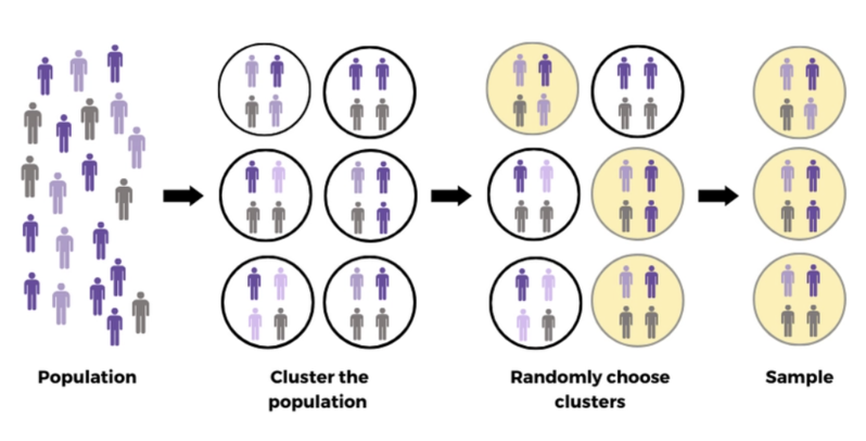
9.6.5 Cluster Sampling

In cluster sampling, the population is divided into naturally occurring groups (clusters), such as households, schools, or city blocks. Instead of sampling individuals across the entire population, you randomly select a few clusters and then measure all or a sample of the units within those selected clusters.

Figure 9.5: Cluster Sampling Process

When to Use:

• When the population is very large and spread out, making it difficult to select a simple random sample from the entire population.

• When cost or logistical constraints make it easier to collect data from a few whole groups rather than scattering your efforts all over the place.

Pros:

Cost-effective and practical when dealing with large, geographically spread-out populations.

Cons:

The variability within clusters can affect precision. If clusters differ greatly from each other, a few selected clusters may not represent the entire population well.

Example Scenario:

Imagine you want to conduct a national health survey. Your population is huge and spread across hundreds of hospitals around the country. Visiting every hospital or sampling patients one by one from all over would be overwhelming and expensive.

Instead, you randomly pick a small number of hospitals (clusters). Within these selected hospitals, you either survey every patient or take a smaller random sample of patients there.

Example Scenario using R:

Now, let’s see how we can simulate this process in R:

set.seed(123)

# Suppose we have 100 hospitals (clusters), each with 50 patients
hospital_id <- rep(1:100, each = 50) # 100 hospitals, each with 50 patients

# Create a data frame of patients, assigning hypothetical health measures:
# Blood Pressure and BMI
patient_df <- data.frame(
  patient_id = 1:5000,
  hospital = hospital_id,
  blood_pressure = rnorm(5000, mean = 120, sd = 15),
  bmi = rnorm(5000, mean = 25, sd = 4)
)

# Randomly select 5 hospitals (clusters) for the study
selected_hospitals <- sample(unique(patient_df$hospital),
  size = 5, replace = FALSE
)

# Extract the data for patients in the selected hospitals
cluster_sample <- patient_df |> filter(hospital %in% selected_hospitals)

cluster_sample |> head()

#>   patient_id hospital blood_pressure      bmi
#> 1        501       11       110.9716 19.57108
#> 2        502       11       105.0945 19.82921
#> 3        503       11       135.4018 18.93117
#> 4        504       11       131.2659 28.43670
#> 5        505       11        97.3625 20.14153
#> 6        506       11       118.5728 27.47622

# Check how many patients we have from each selected hospital

cluster_sample |> count(hospital)

#>   hospital  n
#> 1       11 50
#> 2       24 50
#> 3       50 50
#> 4       59 50
#> 5       95 50

In this example, we use cluster sampling by first selecting 5 hospitals (clusters) from the 100 available. After choosing these clusters, we create a cluster_sample that includes all patients from the selected hospitals. By surveying every patient within these clusters rather than just a subset, we simplify data collection, reduce costs, and focus our efforts on a few representative groups rather than trying to survey patients from every hospital. This approach still allows us to gather valuable information, such as blood pressure and BMI, to better understand the broader population’s health.

9.6.6 Exercise 9.1.3: Cluster Sampling with a Simulated Dataset

In this exercise, you will create a simulated dataset of customers grouped by city. Each city represents a cluster. You will then perform cluster sampling by selecting a few cities and comparing a key characteristic (such as average customer spending) in the sampled clusters versus the entire population.

Steps:

1. Create a simulated dataset of customers, assigning each customer to a city (cluster).

2. Assign some characteristic to each customer (e.g., monthly spending).

3. Randomly select a few cities (clusters).

4. Extract all customers from the selected cities to form your cluster sample.

5. Compare the overall characteristics (e.g., mean monthly spending) of the cluster sample to those of the entire population.

See the Solution to Exercise 9.1.3

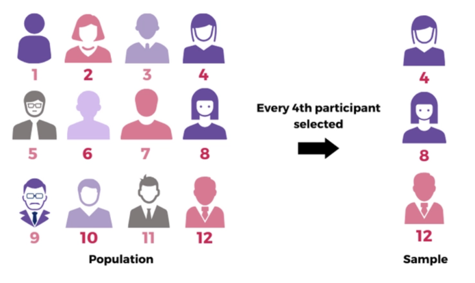
9.6.7 Systematic Sampling

Systematic sampling involves selecting every kth individual from a list or sequence after starting at a random point. For example, if you have a list of 10,000 customers and you need a sample of 500, you would pick every (10000/500) = 20th customer after a random start.

Figure 9.6: Systematic Sampling Process

When to Use:

• When you have a complete list of the population in a random order.

• When it’s easier to pick samples at regular intervals rather than random draws.

Pros:

Simple and efficient once you have a list, and ensures a fairly even spread of the sample across the population.

Cons:

Can introduce bias if the list has a hidden pattern that coincides with the selection interval.

Example Scenario:

Suppose your factory produces 10,000 identical parts in a day (that’s your total population). You want to inspect 500 of these parts to ensure quality—a big enough sample to spot any consistent issues. Rather than randomly stopping the production line and risking inefficiency, you decide to pick every 20th item (10,000/500 = 20) for inspection after a randomly chosen start point between 1 and 20.

Example Scenario using R:

Now, let’s see how to simulate this process in R.

set.seed(123) # Ensure reproducibility

# Suppose the factory produces 10,000 parts a day
total_parts <- 10000

# We want to inspect 500 parts
sample_size <- 500

# Determine the sampling interval (k)
k <- total_parts / sample_size

# Choose a random start point between 1 and k
start <- sample(1:k, 1)

# Create a sequence of parts to inspect: every k-th part starting from 'start'
inspected_parts <- seq(from = start, to = total_parts, by = k)

# Look at the first few part IDs selected
head(inspected_parts)

#> [1]  15  35  55  75  95 115

This systematic approach ensures a steady, predictable pattern: once you set your start, you simply check every 20th part as it comes off the line. By the end of the day, you’ll have a representative sample of 500 parts spaced evenly throughout the entire production run.

9.6.8 Exercise 9.1.4: Systematic Sampling on a Simple List

Use systematic sampling to select individuals from a simple list of IDs (e.g., 1:1000). Your desired sample size is 100. Choose an appropriate interval k, select every kth individual, and verify that the resulting sample follows the intended pattern. Experiment with different values of k to see how the sample changes.

Steps:

1. Create a vector of individuals (e.g., 1:1000).

2. Set the desired sample size to 100.

3. Calculate the interval k (for a list of 1000 individuals and a sample of 100, k = 1000/100 = 10).

4. Randomly select a starting point between 1 and k.

5. Choose every kth element after that starting point.

6. Check that the sample size is correct and that each selection is spaced by k.

7. Experiment with different k values (e.g., 20 or 50) and observe the differences.

See the Solution to Exercise 9.1.4

9.6.9 Practice Quiz 9.1: Probability Sampling

Question 1:

What is the defining feature of probability sampling methods?

1. They always use large sample sizes
   
2. Each member of the population has a known, nonzero chance of selection
   
3. They never require a sampling frame
   
4. They rely on the researcher’s judgment

Question 2:

In simple random sampling (SRS), every member of the population:

1. Has no chance of being selected
   
2. Is selected to represent different subgroups
   
3. Has an equal probability of being selected
   
4. Is chosen based on convenience

Question 3:

Stratified sampling involves:

1. Selecting whole groups at once
   
2. Sampling every kth individual
   
3. Ensuring subgroups are represented proportionally
   
4. Selecting individuals recommended by others

Question 4:

Which method is best if you know certain subgroups (strata) differ and you want each to be represented in proportion to their size?

1. Simple random sampling
   
2. Stratified sampling
   
3. Cluster sampling
   
4. Convenience sampling

Question 5:

Cluster sampling is typically chosen because:

1. It is guaranteed to be perfectly representative
   
2. It reduces cost and logistical complexity
   
3. It involves selecting individuals from every subgroup
   
4. It ensures each individual has the same probability of selection as in SRS

Question 6:

In a national health survey using cluster sampling, which of the following represents a “cluster”?

1. A randomly chosen patient from all over the country
   
2. A randomly selected set of hospitals
   
3. A proportionate sample of age groups
   
4. Every 10th patient in a hospital list

Question 7:

Systematic sampling selects individuals by:

1. Relying on personal judgment
   
2. Selecting every kth individual after a random start
   
3. Dividing the population into strata
   
4. Choosing only those easiest to reach

Question 8:

If the population is 10,000 units and you need a sample of 100, the interval k in systematic sampling is:

1. 10 (10,000 ÷ 1,000)
   
2. 100 (10,000 ÷ 100)
   
3. 20 (10,000 ÷ 500)
   
4. 50 (10,000 ÷ 200)

Question 9:

One advantage of systematic sampling is:

1. It ensures no bias will ever occur
   
2. It provides a convenient and even spread of the sample
   
3. It requires no sampling frame
   
4. It automatically includes all subgroups

Question 10:

Which of the following is NOT a probability sampling method?

1. Simple random sampling
   
2. Stratified sampling
   
3. Cluster sampling
   
4. Convenience sampling

See the Solution to Quiz 9.1

9.7 Experiment 9.2: Non-Probability Sampling Techniques

9.7.1 Convenience Sampling

Convenience sampling involves selecting whichever individuals are easiest to reach. This is a non-probability method, meaning it does not rely on random selection. Because it doesn’t ensure every member of the population has a chance to be selected, it can produce biased results.

Figure 9.7: Convenience Sampling Illustration

When to Use:

• Often used in preliminary studies or quick polls when resources are limited and accuracy is not the top priority.

• When no sampling frame is available, and some data is better than none (with caution).

Pros:

Quick, inexpensive, and easy when you just need preliminary insights.

Cons:

High potential for bias, as the sample may not represent the broader population.

Example Scenario:

A student researcher stands outside the campus cafeteria and surveys the first 50 people who walk out. This approach is simple and fast, but it may not reflect the broader student population’s opinions or habits.

Example Scenario using R:

set.seed(123)
# Suppose we have a dataset of 1,000 students, each with a favorite cafeteria meal
students <- data.frame(
  student_id = 1:1000,
  favorite_meal = sample(c("Pizza", "Salad", "Burger"), 1000, replace = TRUE)
)

# A convenience sample might just be the first 50 students in the dataset
convenience_sample <- head(students, 50)

# Check the distribution of favorite meals in the convenience sample
table(convenience_sample$favorite_meal)

#> 
#> Burger  Pizza  Salad 
#>     19     16     15

Here, the researcher did not randomly select the students. Instead, they simply took whoever was most convenient (the first 50 encountered). While easy, this sample may not accurately represent the entire student body’s meal preferences.

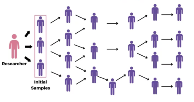
9.7.2 Snowball Sampling

Snowball also known as referral or respondent-driven sampling is used when you have difficulty identifying or accessing members of your target population. In this approach, you start by contacting a few known individuals (called “seeds”) who fit your criteria. These initial participants then refer you to others who share similar characteristics or experiences, and those people, in turn, refer you to still more. This process continues, “snowballing” into a larger sample.

Figure 9.8: Snowball Sampling Process

When to Use:

• When the target population is hidden, rare, or hard to reach (e.g., migrant workers without official registrations, individuals involved in niche subcultures, or certain patient populations).

• When there is no comprehensive sampling frame or list of potential participants.

• Useful in qualitative or exploratory research to gain trust and access through existing social networks.

Pros:

Useful for reaching hidden or hard-to-identify populations (e.g., people in specialized niches or vulnerable communities).

Cons:

Samples may become biased because they rely on social networks and the people your initial contacts know, potentially missing whole segments of the population.

Example Scenario:

You are researching the experiences of freelance data scientists working only on “dark web” analytics—a specialized niche. Identifying such individuals through a public list is almost impossible. You might start with one or two data scientists you know personally, interview them, then ask them to introduce you to colleagues or friends who also fit the criteria.

Example Scenario using R:

In practice, simulating snowball sampling in R might involve having a small “network” or “graph” of individuals and selecting from them based on connections:

set.seed(123)

# Simulate a simple network as a data frame of individuals and their connections
individuals <- data.frame(
  id = 1:20,
  # Each individual is connected to 1-3 others at random
  contacts = I(lapply(1:20, function(x) {
    sample(1:20,
      size = sample(1:3, 1), replace = FALSE
    )
  }))
)

# Start with a known "seed"
seed <- 5

# Get the seed’s contacts
first_wave <- unlist(individuals$contacts[individuals$id == seed])

# Get contacts of the first wave (second wave)
second_wave <- unique(unlist(individuals$contacts[individuals$id %in% first_wave]))

# Combine all waves (excluding duplicates)
snowball_sample_ids <- unique(c(seed, first_wave, second_wave))
snowball_sample_ids

#>  [1]  5  9  3  8 20 17 11 12 15 10

Here, we’ve shown a conceptual approach. In reality, you’d rely on your participants to provide referrals, not just a pre-defined network in code.

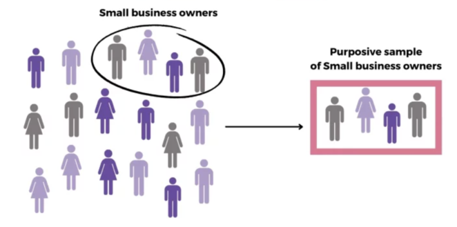
9.7.3 Judgmental (Purposive) Sampling

Judgmental or purposive sampling involves selecting participants based on the researcher’s knowledge, expertise, and judgment. The idea is to choose subjects who are considered to be the most useful or representative to the research study’s aims, rather than randomly.

Figure 9.9: Purposive Sampling Process

When to Use:

• When you want to focus on a particular type of participant who can provide the most relevant information for your research question.

• When you have expert knowledge guiding which subjects are most informative.

• Often used in qualitative research or early-stage exploratory studies.

Pros:

Focuses on key individuals who can provide the richest information.

Cons:

Highly subjective and may reflect researcher bias. Not suitable for drawing generalizable statistical conclusions.

Example Scenario:

A researcher wants to understand high-level strategic decision-making processes within a large biotechnology firm. Rather than interviewing employees from all levels, the researcher decides to focus on those individuals most likely to provide valuable insights into industry trends, company strategy, and organizational challenges—namely the top leadership team.

Example Scenario using R:

Imagine you have a dataset of professionals and their roles:

set.seed(123)
# Suppose we have data on 100 professionals in a biotechnology firm
professionals <- data.frame(
  id = 1:100,
  role = sample(c("CEO", "CTO", "Engineer", "Analyst", "Intern"), 100,
    replace = TRUE
  ),
  # Poisson-distributed years of experience
  years_experience = rpois(100, lambda = 10)
)

professionals |> head()

#>   id     role years_experience
#> 1  1 Engineer                8
#> 2  2 Engineer                8
#> 3  3      CTO                9
#> 4  4      CTO               10
#> 5  5 Engineer               14
#> 6  6   Intern                8

A purposive sample might focus on senior leadership roles that the researcher believes offer the most strategic insights into the industry: CEOs and CTOs.

purposive_sample <- subset(professionals, role %in% c("CEO", "CTO"))

purposive_sample |> head()

#>    id role years_experience
#> 3   3  CTO                9
#> 4   4  CTO               10
#> 8   8  CEO                9
#> 9   9  CTO               11
#> 14 14  CEO                8
#> 16 16  CEO                7

In this example, the researcher chooses participants not by chance, but based on their roles (CEO and CTO) and, indirectly, on their likely longer tenure. While a CEO or CTO may not always have more experience than an Engineer, it’s reasonable to assume that top leadership generally has a wealth of industry insights. This selection method—judgmental or purposive sampling—reflects the researcher’s informed decision about who can provide the most valuable information for the study.

9.7.4 Quota Sampling

Quota sampling involves dividing the population into subgroups based on certain characteristics (such as age groups, gender, or education level) and then non-randomly selecting individuals to meet a pre-set quota that matches these characteristics in proportion to their estimated prevalence in the population. Although similar to stratified sampling in concept, the selection within each subgroup is not random, making it a non-probability technique.

Figure 9.10: Quota Sampling Process

When to Use:

• When you want the sample to reflect certain known proportions of subgroups in the population, but you cannot or do not wish to randomly sample within these strata.

• Often used in market research, opinion polling, or early exploratory surveys where strict probability sampling is not feasible.

Pros:

Ensures representation of certain subgroups, providing more “balanced” samples compared to pure convenience sampling.

Cons:

Still non-random, and the people chosen within each quota are determined by convenience or researcher judgment, potentially introducing bias.

Example Scenario:

A company wants feedback on a new product from a demographic that matches their customer base: \(50\%\) women and \(50\%\) men. Instead of randomly selecting participants, the researcher ensures that interviews continue until they have reached the quota—e.g., 25 women and 25 men—by selecting participants conveniently until quotas are met.

Example Scenario using R:

Now, let’s see how to simulate this process in R.

set.seed(123)
customers <- data.frame(
  id = 1:200,
  gender = sample(c("Male", "Female"), 200, replace = TRUE),
  purchase = sample(c("Yes", "No"), 200, replace = TRUE)
)

Suppose we want a sample of 40 customers, with a quota: 20 Female and 20 Male, We’ll select conveniently (say, the first ones we encounter) until quotas are met.

quota_female <- customers |>
  filter(gender == "Female") |>
  slice(1:20)

quota_male <- customers |>
  filter(gender == "Male") |>
  slice(1:20)

quota_sample <- quota_female |> bind_rows(quota_male)

quota_sample |> count(gender)

#>   gender  n
#> 1 Female 20
#> 2   Male 20

In this simplistic example, we chose the first occurrences (mimicking convenience selection) until each quota was filled.

Reflection Question 3

How can non-probability sampling methods still provide value, even if their findings can’t be easily generalized to the entire population?

9.7.5 Practice Quiz 9.2: Non-Probability Sampling

Question 1:

Non-probability sampling methods are often chosen because:

1. They guarantee generalizable results
   
2. They are cheaper, faster, or more practical
   
3. They eliminate all forms of bias
   
4. They require a complete list of the population

Question 2:

Which method involves selecting participants who are easiest to reach?

1. Convenience sampling
   
2. Snowball sampling
   
3. Purposive sampling
   
4. Quota sampling

Question 3:

Snowball sampling is most useful for:

1. Large, well-documented populations
   
2. Populations where every member is easily identified
   
3. Hidden or hard-to-reach populations
   
4. Ensuring random selection of subgroups

Question 4:

In snowball sampling, the sample grows by:

1. Randomly picking individuals from a list
   
2. Selecting every kth individual
   
3. Asking initial participants to refer others
   
4. Dividing the population into equal parts

Question 5:

Judgmental (purposive) sampling relies on:

1. Each member of the population having an equal chance
   
2. The researcher’s expertise and judgment
   
3. Selecting individuals based solely on their availability
   
4. A systematic interval selection

Question 6:

A researcher who specifically seeks out top experts or key informants in a field is using:

1. Purposive (judgmental) sampling
   
2. Cluster sampling
   
3. Systematic sampling
   
4. Simple random sampling

Question 7:

Quota sampling ensures subgroups are represented by:

1. Randomly selecting from each subgroup
   
2. Matching known proportions but using non-random selection
   
3. Following a strict interval for selection
   
4. Relying on participant referrals

Question 8:

In quota sampling, once you have met the quota for a subgroup:

1. You continue selecting more participants from it anyway
   
2. You stop selecting participants from that subgroup
   
3. You switch to random selection
   
4. You start using a different method

Question 9:

A main drawback of non-probability methods is:

1. They are always expensive
   
2. They cannot measure uncertainty and generalize results easily
   
3. They require a complete list of the population
   
4. They eliminate researcher bias

Question 10:

Which non-probability method would you likely use if you have no sampling frame and need participants quickly, even though it might not be representative?

1. Simple random sampling
   
2. Stratified sampling
   
3. Convenience sampling
   
4. Systematic sampling

See the Solution to Quiz 9.2

9.7.6 Choosing the Right Sampling Technique

Selecting the appropriate sampling technique depends on your research goals, available data, resources, and the need for representativeness.

• Probability-based methods (like simple random, stratified, cluster, and systematic sampling) are generally preferred for statistical inference because they reduce bias and allow for the estimation of sampling error.

• Non-probability methods can be useful for exploratory research, generating hypotheses, or when it’s simply impossible to use a probability sample. However, always be aware of their limitations and be cautious when generalizing findings from these samples.

Reflection Question 4

Think of a scenario where probability sampling would be ideal and another where non-probability sampling would be more realistic. What makes these contexts so different?

9.8 Reproducibility and Ethics

Documenting your sampling decisions, ensuring transparency, and acknowledging limitations are crucial for building trust in your results. Also, consider whether your sampling method might unintentionally exclude or disadvantage certain groups, and think about the ethical implications of doing so.

Reflection Question 5

How could the sampling method you choose affect the fairness and ethics of a study, especially when dealing with sensitive populations or topics?

Reflective Summary

By exploring these techniques, you’ve seen how critical the selection process is in shaping the reliability and fairness of your data-driven insights. Probability sampling offers a path to generalizable, statistically sound conclusions, while non-probability methods provide flexibility, convenience, and creative ways to reach challenging populations—albeit with caution.

Understanding the trade-offs among these methods is key. Armed with these insights, you’re better prepared to design well-structured studies, interpret results accurately, and acknowledge limitations transparently.

What’s Next?

In the next lab, we dive into the Data Science Concept—a culmination of all the techniques you’ve learned in this book. Built upon your skills in data wrangling, visualisation, and statistical concept, this lab will show you how to integrate these methods into a complete, real-world data science workflow.