4  Managing Packages and Workflows

4.1 Introduction

In Lab 4, we will explore essential practices that will enhance your efficiency and effectiveness as an R programmer. You will discover how to extend R’s capabilities by installing and loading packages, how to ensure that your analyses are reproducible by using RStudio Projects, and how to proficiently import and export datasets in various formats. These skills are essential for any data analyst or data scientist, as they enable you to work with a wide range of data sources, maintain the integrity of your analyses, and share your work with others in a consistent and reliable manner.

4.2 Learning Objectives

By the end of this lab, you will be able to:

• Install and Load Packages in R
  Learn how to find, install, and load packages from CRAN and other repositories, thereby extending the functionality of R for your data analysis tasks.

• Ensure Reproducibility with R and RStudio Projects
  Set up and manage RStudio Projects to organise your work, understand the concept of the working directory, and adopt best practices to make your data analyses reproducible and shareable.

• Import and Export Datasets in Various Formats
  Import data into R from different file types, such as CSV, Excel, and SPSS, using appropriate packages and functions. Export your data frames and analysis results to various formats for sharing or reporting.

By completing this lab, you will enhance your ability to manage and analyse data in R more efficiently. You will also ensure that your work is organised, reproducible, and ready to share with others. These foundational skills will support your development as a proficient R programmer and data analyst.

4.3 Prerequisites

Before starting this lab, you should have:

• Completed Lab 3 or have a basic understanding of writing custom functions in R.

• Familiarity with R’s data structures and basic data manipulation.

• An interest in organizing, documenting, and sharing analytical workflows efficiently.

4.4 Understanding Packages and Libraries in R

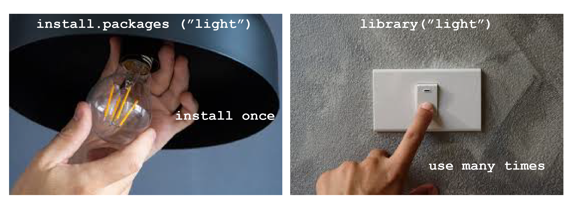
In R, a package is a collection of functions, data, and code that extends the basic functionality of R. Think of it as a specialised toolkit for particular tasks or topics. For example, packages like tidyr and janitor facilitate data wrangling, while others focus on graphics, modelling, or data import and export.

A library is a location on your computer’s file system where installed packages are stored. When you install a package, it is saved in a library so that you can easily access it in future R sessions.

4.5 Compiling R Packages from Source

You may occasionally need additional tools to compile R packages from source, depending on your operating system:

• Windows

  Windows does not support code compilation natively. Therefore, you need Rtools, which provides the necessary software, including compilers and libraries, to build R packages from source. You can download Rtools from CRAN: https://cran.rstudio.com/bin/windows/Rtools/. After installing the appropriate version of Rtools, R will automatically detect it.

  Note

  To check your R version, run the following code in your console:

  R.version

  To verify that Rtools is correctly installed, you can run the following code in your console:

  Sys.which("make")

• Mac OS

  On macOS, you need the Xcode Command Line Tools, which provide similar capabilities to Rtools on Windows. You can install Xcode from the Mac App Store:

  http://itunes.apple.com/us/app/xcode/id497799835?mt=12 or install the Command Line Tools directly by running:

  xcode-select --install

• Linux

  Most Linux distributions already come with the necessary tools for compiling packages. If additional developer tools are needed, you can install them via your package manager, usually by installing packages like build-essential or similar for your Linux distribution.

  Note

  On Debian/Ubuntu, you can install the essential software for R package development and LaTeX (if needed for documentation) with:

  sudo apt-get install r-base-dev texlive-full

  To ensure all dependencies for building R itself from source are met, you can run:

  sudo apt-get build-dep r-base-core

4.6 Experiment 4.1: Installing and Loading Packages

As you progress in R, you will frequently need functions that are not included in the base R installation. These are provided by packages, which you can easily install and load into your R environment.

4.6.1 Installing Packages from CRAN

The Comprehensive R Archive Network (CRAN) hosts thousands of packages. To install a package from CRAN, use:

install.packages("package_name")

Note

Replace package_name with the name of the package you want to install.

For example, to install the tidyverse package, use:

install.packages("tidyverse")

Similarly, to install the janitor package, use:

install.packages("janitor")

Warning

Remember to enclose the package name in quotes—either double ("package_name") or single ('package_name').

4.6.2 Installing Packages from External Repositories

Some packages may not be available on CRAN but can be installed from GitHub or GitLab. First, install a helper package such as devtools or remotes:

install.packages("devtools")
# or
install.packages("remotes")

Then, to install a package from GitHub, for example openintro package, use:

devtools::install_github("OpenIntroStat/openintro")
# or
remotes::install_github("OpenIntroStat/openintro")

You can also install development versions of packages using these helper packages. For instance:

#|
remotes::install_github("datalorax/equatiomatic")

4.6.3 Loading Packages

Once a package has been installed, you need to load it into your R session to use its functions. You can do this by calling the library() function, as demonstrated in the code cell below:

library(package_name)

Here, package_name refers to the specific package you want to load into the R environment. For example, to load the tidyverse package:

library(tidyverse)

#> ── Attaching core tidyverse packages ──────────────────────── tidyverse 2.0.0 ──
#> ✔ dplyr     1.1.4     ✔ readr     2.1.5
#> ✔ forcats   1.0.0     ✔ stringr   1.5.1
#> ✔ ggplot2   3.5.1     ✔ tibble    3.2.1
#> ✔ lubridate 1.9.3     ✔ tidyr     1.3.1
#> ✔ purrr     1.0.2     
#> ── Conflicts ────────────────────────────────────────── tidyverse_conflicts() ──
#> ✖ dplyr::filter() masks stats::filter()
#> ✖ dplyr::lag()    masks stats::lag()
#> ℹ Use the conflicted package (<http://conflicted.r-lib.org/>) to force all conflicts to become errors

This command loads core tidyverse packages essential for most data analysis project¹. Other installed packages can also be loaded in such manner:

library(janitor)

library(bulkreadr)

If you run this code and get the error message there is no package called "bulkreadr", you’ll need to first install it, then run library() once again.

install.packages("bulkreadr")

library(bulkreadr)

Tip

You only need to install a package once, but you must load it each time you start a new R session.

Figure 4.1: Installing vs. Loading Packages in R

4.6.4 Using Functions from a Package

When working with R packages, there are two primary ways to use a function from a package:

1. Load the Package and Call the Function Directly

You can load the package into your R session using the library() function, and then call the desired function by its name. For example:

#|
# Load the janitor package
library(janitor)

# Use the clean_names() function
clean_names(iris)

#> # A tibble: 150 × 5
#>    sepal_length sepal_width petal_length petal_width species
#>           <dbl>       <dbl>        <dbl>       <dbl> <fct>  
#>  1          5.1         3.5          1.4         0.2 setosa 
#>  2          4.9         3            1.4         0.2 setosa 
#>  3          4.7         3.2          1.3         0.2 setosa 
#>  4          4.6         3.1          1.5         0.2 setosa 
#>  5          5           3.6          1.4         0.2 setosa 
#>  6          5.4         3.9          1.7         0.4 setosa 
#>  7          4.6         3.4          1.4         0.3 setosa 
#>  8          5           3.4          1.5         0.2 setosa 
#>  9          4.4         2.9          1.4         0.2 setosa 
#> 10          4.9         3.1          1.5         0.1 setosa 
#> # ℹ 140 more rows

In this approach, you only need to load the package once in your session, and then you can use its functions without specifying the package name.

2. Use the :: Operator to Call the Function Without Loading the Package

The :: operator is used to call a function from a specific package without loading the entire package into your R session. This is particularly useful when:

• Avoiding Namespace Conflicts: If multiple packages have functions with the same name, :: ensures you use the correct one.

• Improving Code Clarity: It makes your code more readable by clearly indicating which package a function comes from.

• Reducing Memory Usage: Only the specific function is accessed, not the entire package.

The syntax is:

packageName::functionName(arguments)

where:

• packageName: The name of the package where the function resides.

• functionName: The specific function you want to use from the package.

Example

# Using the double colon to access clean_names() from janitor package
janitor::clean_names(iris)

#> # A tibble: 150 × 5
#>    sepal_length sepal_width petal_length petal_width species
#>           <dbl>       <dbl>        <dbl>       <dbl> <fct>  
#>  1          5.1         3.5          1.4         0.2 setosa 
#>  2          4.9         3            1.4         0.2 setosa 
#>  3          4.7         3.2          1.3         0.2 setosa 
#>  4          4.6         3.1          1.5         0.2 setosa 
#>  5          5           3.6          1.4         0.2 setosa 
#>  6          5.4         3.9          1.7         0.4 setosa 
#>  7          4.6         3.4          1.4         0.3 setosa 
#>  8          5           3.4          1.5         0.2 setosa 
#>  9          4.4         2.9          1.4         0.2 setosa 
#> 10          4.9         3.1          1.5         0.1 setosa 
#> # ℹ 140 more rows

The clean_names() function, in this case, returns the iris data frame with column names formatted in a consistent and clean style.

Tip

Ensure that the janitor package is installed before using its functions. If it’s not installed, you can install it using install.packages(“janitor”).

As shown in Table 4.1, using library() attaches the entire package, while the :: operator allows you to call specific functions without loading the entire package. This difference can significantly impact memory usage and clarity in your scripts, especially when you’re only using a few functions from a large package.

Table 4.1: Comparing library() and :: Operator

Aspect	library()	:: Operator
Loading Behavior	Attaches the entire package to the session	Accesses specific functions without loading the package
Namespace Conflicts	Potential for conflicts if multiple packages have functions with the same name	Avoids conflicts by specifying the package
Memory Usage	Loads all exported objects, increasing memory usage	Minimal memory usage as only specific functions are accessed
Code Verbosity	Less verbose; functions can be called directly	More verbose; requires prefixing with package name
Use Cases	When using multiple functions from a package extensively	When using only a few functions or to avoid conflicts

4.6.5 Practice Quiz 4.1

Question 1:

Imagine that you want to install the shiny package from CRAN. Which command should you use?

1. install.packages("shiny")
2. library("shiny")
   
3. install.packages(shiny)
   
4. require("shiny")

Question 2:

What must you do after installing a package before you can use it in your current session?

1. Restart R
   
2. Run install.packages() again
   
3. Load it with library()
   
4. Convert the package into a dataset

Question 3:

If you want to install a package that is not on CRAN (e.g., from GitHub), which additional package would be helpful?

1. installer
   
2. rio
   
3. devtools
   
4. github_install

Question 4:

Which function would you use to update all outdated packages in your R environment?

1. update.packages()
   
2. install.packages()
   
3. library()
   
4. require()

Question 5:

Which function can be used to check the version of an installed package?

1. version()
   
2. packageVersion()
   
3. libraryVersion()
   
4. install.packages()

See the Solution to Quiz 4.1

4.7 Experiment 4.2: Ensuring Reproducibility with R and RStudio Projects

Reproducibility is vital in data science. It allows analyses to be revisited, results to be verified, and insights to be shared seamlessly, whether with collaborators or for future reference. With R and RStudio Projects, you can create a self-contained workspace that keeps your work organised and reproducible.

4.7.1 Working Directory and Paths

Your working directory is where R looks for files to read and where it saves outputs. You can find your current working directory in two ways:

1. In the Console: At the top of the RStudio console, the current working directory is displayed.

   

2. Using Code: Run the following command:

   getwd()

   [1] "C:/Users/Ezekiel Adebayo/Desktop/stock-market"

   If you’re not using an RStudio project, you’ll need to set the working directory manually each time. For instance:

   setwd("/path/to/your/data_analysis")

   Tip

   You can use the keyboard shortcut Ctrl + Shift + H in RStudio to quickly choose your working directory.

• Absolute Paths: Start from the root of your file system (e.g., C:/Users/YourName/Documents/data.csv). These paths are specific to your computer and should be avoided in shared scripts.

• Relative Paths: Refer to files relative to your working directory (e.g., data/data.csv). Using relative paths ensures portability and makes your scripts easier to share and reuse.

4.7.2 RStudio Projects

RStudio Projects provide a centralised environment for all your analyses: data files, scripts, figures, outputs, and documentation. This setup ensures your work remains organised, consistent, and reproducible.

Benefits of RStudio Projects

1. Organisation
   All project files are stored in one place, making it easy to navigate and manage.

2. Relative Paths
   RStudio automatically sets the working directory to the project folder, allowing you to use relative paths (e.g., data/my_data.csv). This eliminates the need for hardcoding absolute paths, ensuring your code works on any system.

3. Consistency Across Systems
   When you open your RStudio project on another computer, it recognises the same folder structure, making your work portable and adaptable.

4. Reproducibility
   With all components centralised and paths consistent, RStudio Projects enable others to replicate your workflow effortlessly. Everything needed to reproduce your analysis is neatly packaged and ready to go.

4.7.3 How RStudio Projects Organize Your Work

When you set up an RStudio Project, it acts as the root folder for your analysis. A recommended structure is shown in Figure 4.2 below:

Figure 4.2: Practical Framework for Reproducible Data Analysis with RStudio Projects.

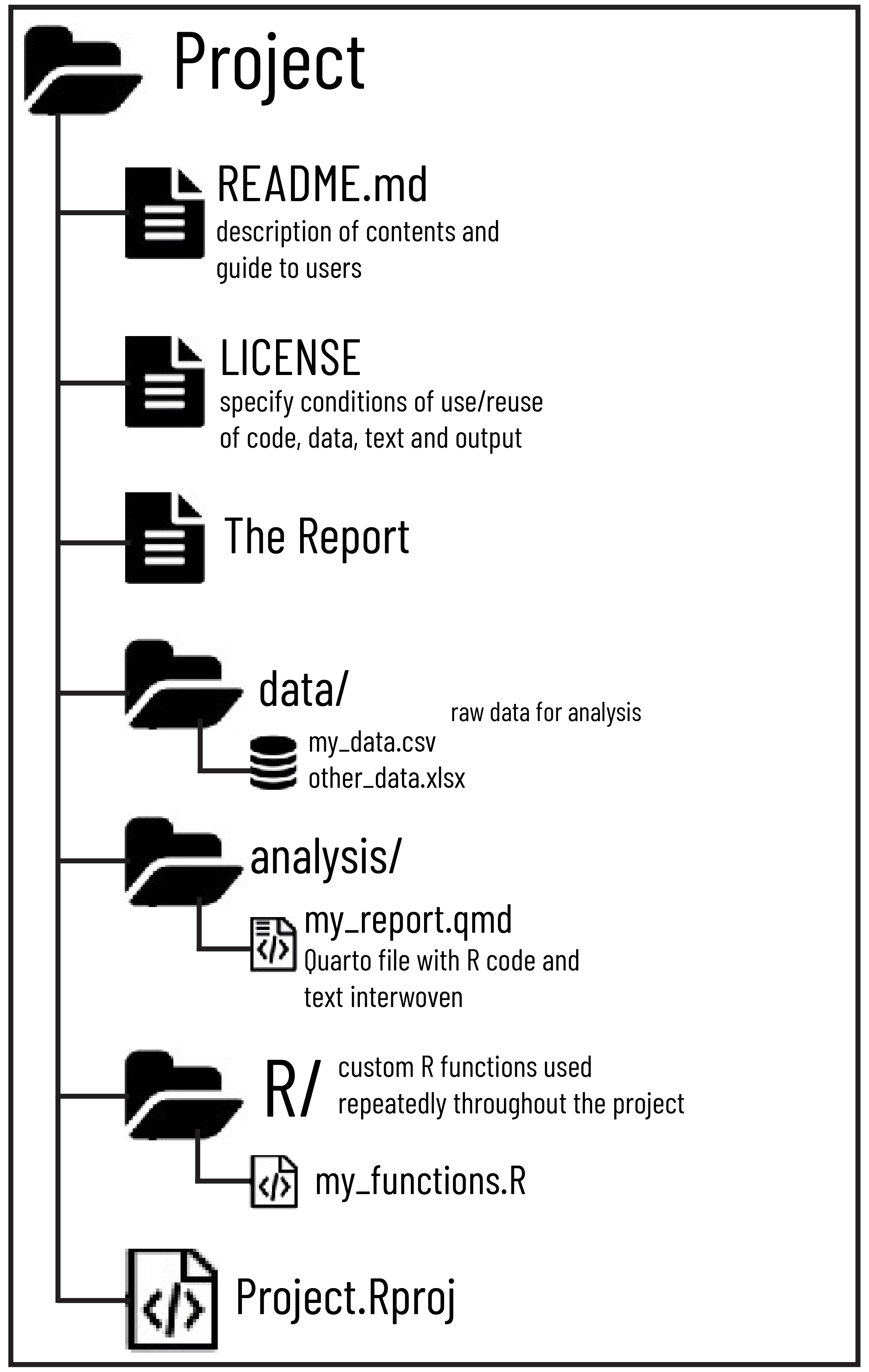
• Top-Level Files
  Files like README.md provide an overview of the project, while a LICENSE file outlines terms of use for the code and data. These files are essential for collaboration and transparency.

• Data Folder (data/)
  This folder contains raw data files in formats like .csv or .xlsx. Raw data is stored here in its original state to preserve reproducibility.

• Analysis Folder (analysis/)
  Scripts or dynamic documents, such as Quarto files (.qmd) or R Markdown files (.Rmd), go here. These documents combine R code, narrative text, and visualizations, serving as the heart of your analysis.

• Custom Functions Folder (R/)
  Reusable R scripts containing custom functions are saved here. These can be sourced into analysis scripts to keep your workflow modular and efficient.

This structure, combined with relative paths, ensures a clean, logical, and reproducible workflow.

4.7.4 Setting Up Your RStudio Project

Let’s create a new RStudio project. You can do this by following these simple steps:

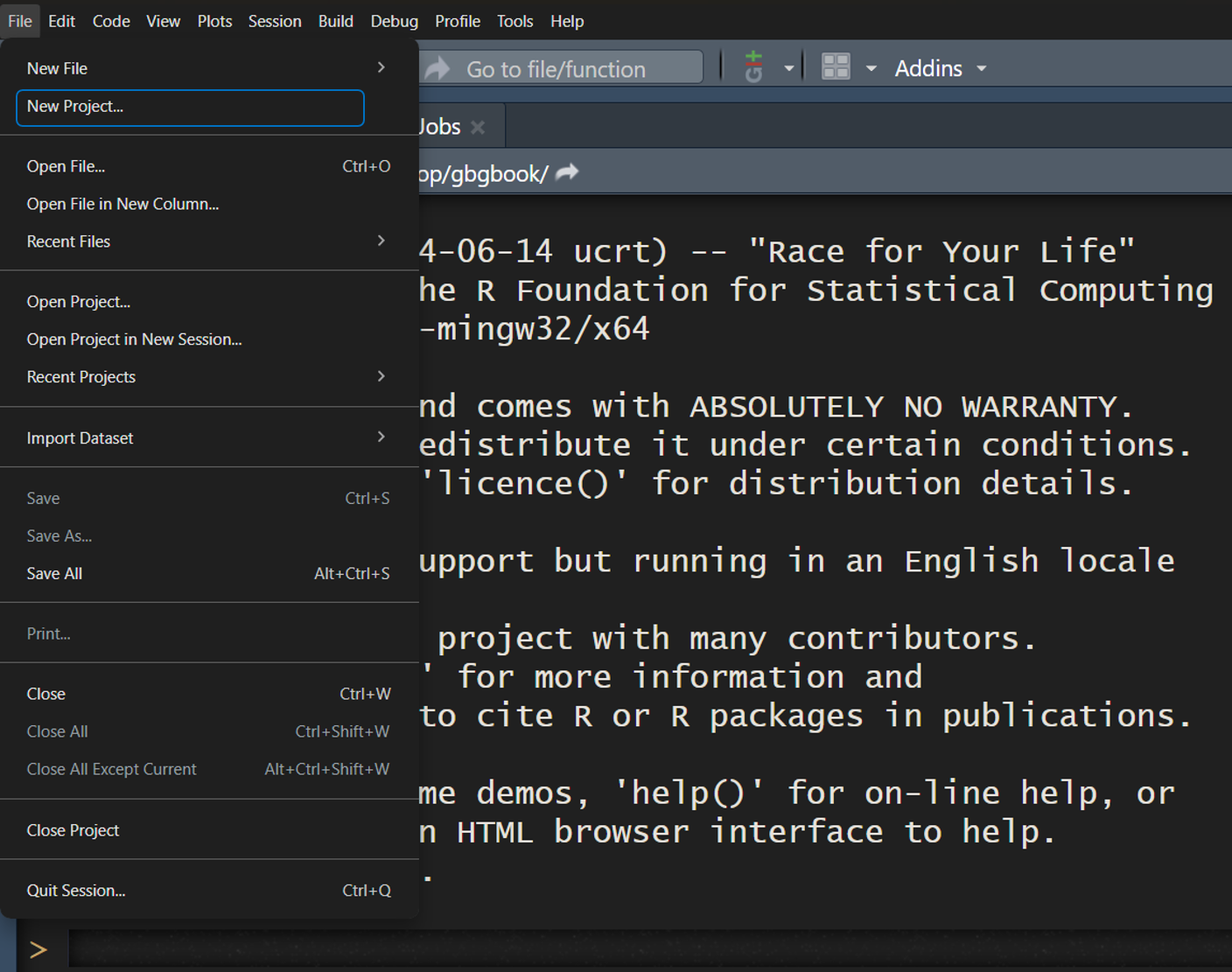
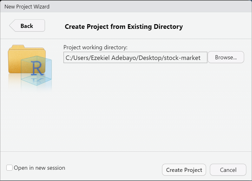
4.7.4.1 Step 1: Create a New Project

1. Go to: File → New Project in RStudio

Figure 4.3: Creating a New Project in RStudio

2. Choose: Existing Directory

Figure 4.4: Creating a New Project in RStudio

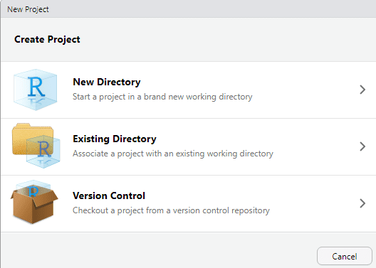
3. Select the folder you want to use as your project’s working directory and RStudio will create a project file (.Rproj).

4. Click: Create Project

Figure 4.5: Creating a New R Project from an Existing Directory

Once you click “Create Project”, you’re all set! You’ll be inside your new RStudio project.

Figure 4.6: RStudio Project: Stock Market Price Scraper Using R

4.7.4.2 Step 2: Arrange Your Files

Organise your project files into the following structure:

• data/: Store raw data files here in formats such as .csv or .xlsx.

• analysis/: Place your analysis scripts or reports in this folder. For example, you might use a Quarto file (my_report.qmd) to combine R code, narrative text, and visualisations.

• R/: Save reusable R functions in this folder, and source them into your scripts as needed.

4.7.4.3 Step 3: Use Relative Paths

Always refer to files using paths relative to your project folder. For example:

data <- read.csv("data/my_data.csv")

4.7.4.4 Step 4: Add Documentation

Include a README.md file to document the purpose, structure, and usage of your project. Add a LICENSE file to define terms of use.

Figure 4.7: Organization of an R Project Directory

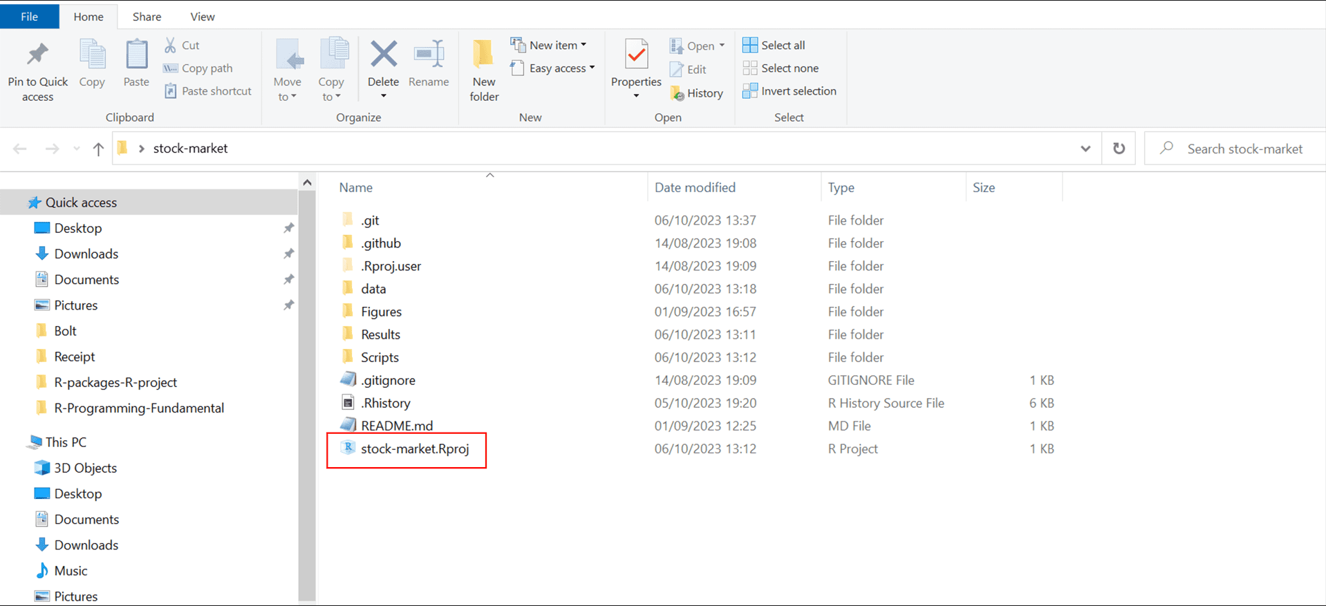
From now on, whenever you open this project (by clicking the .Rproj file), RStudio will automatically set your working directory, allowing you to use relative paths easily as shown in Figure 4.7

4.7.5 Practice Quiz 4.2

Question 1:

What is a key advantage of using RStudio Projects?

1. They automatically install packages.
   
2. They allow you to use absolute paths easily.
   
3. They set the working directory to the project folder, enabling relative paths.
   
4. They prevent package updates.

Question 2:

Which file extension identifies an RStudio Project file?

1. .Rdata
   
2. .Rproj
   
3. .Rmd
   
4. .Rscript

Question 3:

Why are relative paths preferable in a collaborative environment?

1. They are shorter and easier to type.
   
2. They change automatically when you move files.
   
3. They ensure that the code works regardless of the user’s file system structure.
   
4. They are required for Git version control.

See the Solution to Quiz 4.2

4.8 Experiment 4.3: Importing and Exporting Data in R

Data import and export are vital steps in data science. With R, you can load data from spreadsheets, databases, and many other formats, and subsequently save your processed results. Figure 4.8 below illustrates some popular R packages for data import:

Figure 4.8: Data Import Packages in R

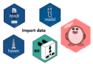
Note

Packages like readr, readxl, and haven are part of the tidyverse, and therefore are pre-installed when you install the tidyverse. You do not need to install these packages individually. For a complete list of tidyverse packages, see the following code:

tidyverse::tidyverse_packages()

#>  [1] "broom"         "conflicted"    "cli"           "dbplyr"       
#>  [5] "dplyr"         "dtplyr"        "forcats"       "ggplot2"      
#>  [9] "googledrive"   "googlesheets4" "haven"         "hms"          
#> [13] "httr"          "jsonlite"      "lubridate"     "magrittr"     
#> [17] "modelr"        "pillar"        "purrr"         "ragg"         
#> [21] "readr"         "readxl"        "reprex"        "rlang"        
#> [25] "rstudioapi"    "rvest"         "stringr"       "tibble"       
#> [29] "tidyr"         "xml2"          "tidyverse"

You don’t need to install any of these packages individually since they’re all included with the tidyverse installation.

R offers some excellent packages that simplify the processes of importing and exporting data. In the sections below, we will explore a few commonly used packages and functions that are essential when working with data in R.

4.8.1 Flat Files

Flat files, such as CSV files, are among the most common formats for data storage and exchange. The readr package (a core component of the tidyverse) provides functions specifically designed to handle flat files. The two primary functions are:

• read_csv(): This function imports data from a CSV file into R as a data frame, akin to loading data directly from a spreadsheet.

• write_csv(): Once your data analysis is complete, this function exports your data frame to a CSV file. It is particularly useful for sharing your results or maintaining a backup.

Example 1: Reading CSV Data From a File

Suppose you have a file named cleveland-heart-disease-database.csv located in the r-data folder. You can import this flat file into R as follows:

library(tidyverse)

heart_disease_data <- read_csv("r-data/cleveland-heart-disease-database.csv")

heart_disease_data

#> # A tibble: 303 × 14
#>      age sex    `chest pain type` resting blood pressur…¹ serum cholestoral in…²
#>    <dbl> <chr>  <chr>                               <dbl>                  <dbl>
#>  1    63 male   typical angina                        145                    233
#>  2    67 male   asymptomatic                          160                    286
#>  3    67 male   asymptomatic                          120                    229
#>  4    37 male   non-anginal pain                      130                    250
#>  5    41 female atypical angina                       130                    204
#>  6    56 male   atypical angina                       120                    236
#>  7    62 female asymptomatic                          140                    268
#>  8    57 female asymptomatic                          120                    354
#>  9    63 male   asymptomatic                          130                    254
#> 10    53 male   asymptomatic                          140                    203
#> # ℹ 293 more rows
#> # ℹ abbreviated names: ¹​`resting blood pressure in mm Hg`,
#> #   ²​`serum cholestoral in mg/dl`
#> # ℹ 9 more variables: `fasting blood sugar > 120 mg/dl` <lgl>,
#> #   `resting electrocardiographic results` <dbl>,
#> #   `maximum heart rate achieved` <dbl>, `exercise induced angina` <chr>,
#> #   `ST depression` <dbl>, `slope of the peak exercise ST segment` <chr>, …

Tip

For information on downloading the data, please refer to Appendix B.1. Should you encounter any errors when executing the code, first set up your RStudio project as described in Section 4.8.5, then re-run the code.

When you run read_csv(), you will notice a message detailing the number of rows and columns, the delimiter used, and information regarding the column types. This ensures that your data is read correctly. You may also specify how missing values are represented via the na argument. For example, setting na = "?" tells read_csv() to treat the ? symbol as NA in the dataset:

heart_disease_data <- read_csv("r-data/cleveland-heart-disease-database.csv", na = "?")

heart_disease_data

#> # A tibble: 303 × 14
#>      age sex    `chest pain type` resting blood pressur…¹ serum cholestoral in…²
#>    <dbl> <chr>  <chr>                               <dbl>                  <dbl>
#>  1    63 male   typical angina                        145                    233
#>  2    67 male   asymptomatic                          160                    286
#>  3    67 male   asymptomatic                          120                    229
#>  4    37 male   non-anginal pain                      130                    250
#>  5    41 female atypical angina                       130                    204
#>  6    56 male   atypical angina                       120                    236
#>  7    62 female asymptomatic                          140                    268
#>  8    57 female asymptomatic                          120                    354
#>  9    63 male   asymptomatic                          130                    254
#> 10    53 male   asymptomatic                          140                    203
#> # ℹ 293 more rows
#> # ℹ abbreviated names: ¹​`resting blood pressure in mm Hg`,
#> #   ²​`serum cholestoral in mg/dl`
#> # ℹ 9 more variables: `fasting blood sugar > 120 mg/dl` <lgl>,
#> #   `resting electrocardiographic results` <dbl>,
#> #   `maximum heart rate achieved` <dbl>, `exercise induced angina` <chr>,
#> #   `ST depression` <dbl>, `slope of the peak exercise ST segment` <chr>, …

Example 2: Writing to a CSV File

After processing or analysing your data, you might wish to save your results. The write_csv() function writes the data to disk, enabling you to share your cleaned or transformed data with others. The key arguments are:

• x: The data frame to be saved.

• file: the destination file path.

For example:

write_csv(heart_disease_data, "processed-cleveland-heart-disease-data.csv")

Tip

Additional arguments allow you to control the representation of missing values (using na) and whether to append to an existing file (using append). For instance:

4.8.2 Spreadsheets

Microsoft Excel is a widely used application that organises data into worksheets within a single workbook². The readxl package is used to import Excel spreadsheets (e.g. .xlsx files) into R, while the writexl package is used to export data frames to Excel files.

The primary functions are:

• read_xlsx(): Imports an Excel file into R. You can specify the worksheet containing your data by using the sheet argument.

• write_xlsx(): Export your data frame to an Excel file—ideal for sharing your work with colleagues who prefer Excel.

Example 1: Reading Excel Spreadsheets

In this example, we import data from an Excel spreadsheet using the readxl package. Although readxl is not part of the core tidyverse, it is installed automatically with the tidyverse, so you must load it explicitly:

library(tidyverse)
library(readxl)
library(writexl)

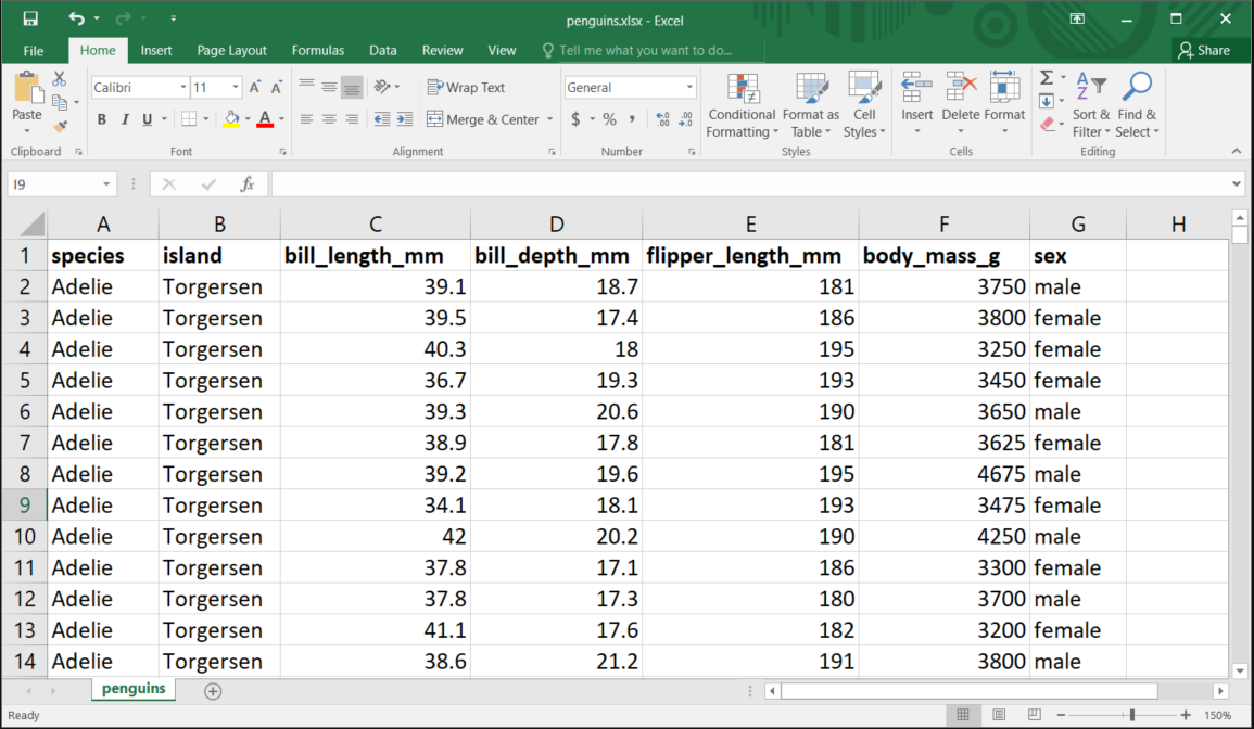
The spreadsheet, as shown in Figure 4.9, can be downloaded from https://docs.google.com/spreadsheets/d/107H-n59gDw0QoIktksU9wv6Iro4TGUAOgmQJW6pb19Y

Figure 4.9: Spreadsheet called penguins.xlsx in Excel.

The first argument of read_xlsx() is the file path:

penguins <- read_xlsx("r-data/penguins.xlsx")

This function reads the file as a tibble³:

penguins

#> # A tibble: 337 × 7
#>    species island    bill_length_mm bill_depth_mm flipper_length_mm body_mass_g
#>    <chr>   <chr>              <dbl>         <dbl>             <dbl>       <dbl>
#>  1 Adelie  Torgersen           39.1          18.7               181        3750
#>  2 Adelie  Torgersen           39.5          17.4               186        3800
#>  3 Adelie  Torgersen           40.3          18                 195        3250
#>  4 Adelie  Torgersen           36.7          19.3               193        3450
#>  5 Adelie  Torgersen           39.3          20.6               190        3650
#>  6 Adelie  Torgersen           38.9          17.8               181        3625
#>  7 Adelie  Torgersen           39.2          19.6               195        4675
#>  8 Adelie  Torgersen           34.1          18.1               193        3475
#>  9 Adelie  Torgersen           42            20.2               190        4250
#> 10 Adelie  Torgersen           37.8          17.1               186        3300
#> # ℹ 327 more rows
#> # ℹ 1 more variable: sex <chr>

This dataset contains data on 337 penguins and includes seven variables for each species.

Example 2: Reading Worksheets

Spreadsheets may contain multiple worksheets. Figure 4.10 illustrates an Excel workbook with several sheets. The data, sourced from the ggplot2 package, is available at https://docs.google.com/spreadsheets/d/1izO0mHu3L9AMySQUXGDn9GPs1n-VwGFSEoAKGhqVQh0. Each worksheet contains information on diamond prices for different cuts.

Figure 4.10: Spreadsheet called diamond.xlsx in Excel.

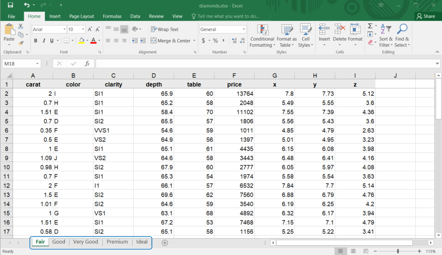
You can read a specific worksheet by using the sheet argument in read_xlsx(). By default, the first worksheet is read.

diamonds_fair <- read_xlsx("r-data/diamonds.xlsx", sheet = "Fair")

diamonds_fair

#> # A tibble: 60 × 9
#>    carat color clarity depth table price     x     y     z
#>    <dbl> <chr> <chr>   <dbl> <dbl> <dbl> <dbl> <dbl> <dbl>
#>  1  2    I     SI1      65.9    60 13764  7.8   7.73  5.12
#>  2  0.7  H     SI1      65.2    58  2048  5.49  5.55  3.6 
#>  3  1.51 E     SI1      58.4    70 11102  7.55  7.39  4.36
#>  4  0.7  D     SI2      65.5    57  1806  5.56  5.43  3.6 
#>  5  0.35 F     VVS1     54.6    59  1011  4.85  4.79  2.63
#>  6  0.5  E     VS2      64.9    56  1397  5.01  4.95  3.23
#>  7  1    E     SI1      65.1    61  4435  6.15  6.08  3.98
#>  8  1.09 J     VS2      64.6    58  3443  6.48  6.41  4.16
#>  9  0.98 H     SI2      67.9    60  2777  6.05  5.97  4.08
#> 10  0.7  F     SI1      65.3    54  1974  5.58  5.54  3.63
#> # ℹ 50 more rows

If numerical data is read as text because the string “NA” is not automatically recognised as a missing value, you may correct this by specifying the na argument:

read_excel("r-data/diamonds.xlsx", sheet = "Fair", na = "NA")

#> # A tibble: 60 × 9
#>    carat color clarity depth table price     x     y     z
#>    <dbl> <chr> <chr>   <dbl> <dbl> <dbl> <dbl> <dbl> <dbl>
#>  1  2    I     SI1      65.9    60 13764  7.8   7.73  5.12
#>  2  0.7  H     SI1      65.2    58  2048  5.49  5.55  3.6 
#>  3  1.51 E     SI1      58.4    70 11102  7.55  7.39  4.36
#>  4  0.7  D     SI2      65.5    57  1806  5.56  5.43  3.6 
#>  5  0.35 F     VVS1     54.6    59  1011  4.85  4.79  2.63
#>  6  0.5  E     VS2      64.9    56  1397  5.01  4.95  3.23
#>  7  1    E     SI1      65.1    61  4435  6.15  6.08  3.98
#>  8  1.09 J     VS2      64.6    58  3443  6.48  6.41  4.16
#>  9  0.98 H     SI2      67.9    60  2777  6.05  5.97  4.08
#> 10  0.7  F     SI1      65.3    54  1974  5.58  5.54  3.63
#> # ℹ 50 more rows

Another approach is to use excel_sheets() to list all the worksheets in an Excel file and then import only the ones you need.

excel_sheets("r-data/diamonds.xlsx")

#> [1] "Fair"      "Good"      "Very Good" "Premium"   "Ideal"

Once the worksheet names are known, they can be imported individually:

diamonds_fair <- read_excel("r-data/diamonds.xlsx", sheet = "Fair")

diamonds_good <- read_excel("r-data/diamonds.xlsx", sheet = "Good")

diamonds_very_good <- read_excel("r-data/diamonds.xlsx", sheet = "Very Good")

diamonds_premium <- read_excel("r-data/diamonds.xlsx", sheet = "Premium")

diamonds_ideal <- read_excel("r-data/diamonds.xlsx", sheet = "Ideal")

In this instance, the complete diamonds dataset is distributed across five worksheets that share the same columns but differ in the number of rows. You can inspect their dimensions using:

dim(diamonds_fair)

#> [1] 60  9

dim(diamonds_good)

#> [1] 49  9

dim(diamonds_very_good)

#> [1] 42  9

dim(diamonds_premium)

#> [1] 49  9

dim(diamonds_ideal)

#> [1] 60  9

You can also combine the worksheets into one data frame by using bind_rows():

diamonds <- bind_rows(
  diamonds_fair,
  diamonds_good,
  diamonds_very_good,
  diamonds_premium,
  diamonds_ideal
)

diamonds

#> # A tibble: 260 × 9
#>    carat color clarity depth table price     x     y     z
#>    <dbl> <chr> <chr>   <dbl> <dbl> <dbl> <dbl> <dbl> <dbl>
#>  1  2    I     SI1      65.9    60 13764  7.8   7.73  5.12
#>  2  0.7  H     SI1      65.2    58  2048  5.49  5.55  3.6 
#>  3  1.51 E     SI1      58.4    70 11102  7.55  7.39  4.36
#>  4  0.7  D     SI2      65.5    57  1806  5.56  5.43  3.6 
#>  5  0.35 F     VVS1     54.6    59  1011  4.85  4.79  2.63
#>  6  0.5  E     VS2      64.9    56  1397  5.01  4.95  3.23
#>  7  1    E     SI1      65.1    61  4435  6.15  6.08  3.98
#>  8  1.09 J     VS2      64.6    58  3443  6.48  6.41  4.16
#>  9  0.98 H     SI2      67.9    60  2777  6.05  5.97  4.08
#> 10  0.7  F     SI1      65.3    54  1974  5.58  5.54  3.63
#> # ℹ 250 more rows

An alternative method to import all worksheets from a workbook is provided by the read_excel_workbook() function from the bulkreadr package. This function reads the data from every sheet in an Excel workbook and returns a single appended data frame:

library(bulkreadr)

diamonds <- read_excel_workbook("r-data/diamonds.xlsx")

diamonds

#> # A tibble: 260 × 9
#>    carat color clarity depth table price     x     y     z
#>    <dbl> <chr> <chr>   <dbl> <dbl> <dbl> <dbl> <dbl> <dbl>
#>  1  2    I     SI1      65.9    60 13764  7.8   7.73  5.12
#>  2  0.7  H     SI1      65.2    58  2048  5.49  5.55  3.6 
#>  3  1.51 E     SI1      58.4    70 11102  7.55  7.39  4.36
#>  4  0.7  D     SI2      65.5    57  1806  5.56  5.43  3.6 
#>  5  0.35 F     VVS1     54.6    59  1011  4.85  4.79  2.63
#>  6  0.5  E     VS2      64.9    56  1397  5.01  4.95  3.23
#>  7  1    E     SI1      65.1    61  4435  6.15  6.08  3.98
#>  8  1.09 J     VS2      64.6    58  3443  6.48  6.41  4.16
#>  9  0.98 H     SI2      67.9    60  2777  6.05  5.97  4.08
#> 10  0.7  F     SI1      65.3    54  1974  5.58  5.54  3.63
#> # ℹ 250 more rows

You can also specify the .id argument in read_excel_workbook() to add an output column that identifies the source of each row (using either the sheet names or their positions):

diamonds <- bulkreadr::read_excel_workbook("r-data/diamonds.xlsx", .id = "sheet")

diamonds

#> # A tibble: 260 × 10
#>    sheet carat color clarity depth table price     x     y     z
#>    <chr> <dbl> <chr> <chr>   <dbl> <dbl> <dbl> <dbl> <dbl> <dbl>
#>  1 Fair   2    I     SI1      65.9    60 13764  7.8   7.73  5.12
#>  2 Fair   0.7  H     SI1      65.2    58  2048  5.49  5.55  3.6 
#>  3 Fair   1.51 E     SI1      58.4    70 11102  7.55  7.39  4.36
#>  4 Fair   0.7  D     SI2      65.5    57  1806  5.56  5.43  3.6 
#>  5 Fair   0.35 F     VVS1     54.6    59  1011  4.85  4.79  2.63
#>  6 Fair   0.5  E     VS2      64.9    56  1397  5.01  4.95  3.23
#>  7 Fair   1    E     SI1      65.1    61  4435  6.15  6.08  3.98
#>  8 Fair   1.09 J     VS2      64.6    58  3443  6.48  6.41  4.16
#>  9 Fair   0.98 H     SI2      67.9    60  2777  6.05  5.97  4.08
#> 10 Fair   0.7  F     SI1      65.3    54  1974  5.58  5.54  3.63
#> # ℹ 250 more rows

Example 3: Writing Data to an Excel File

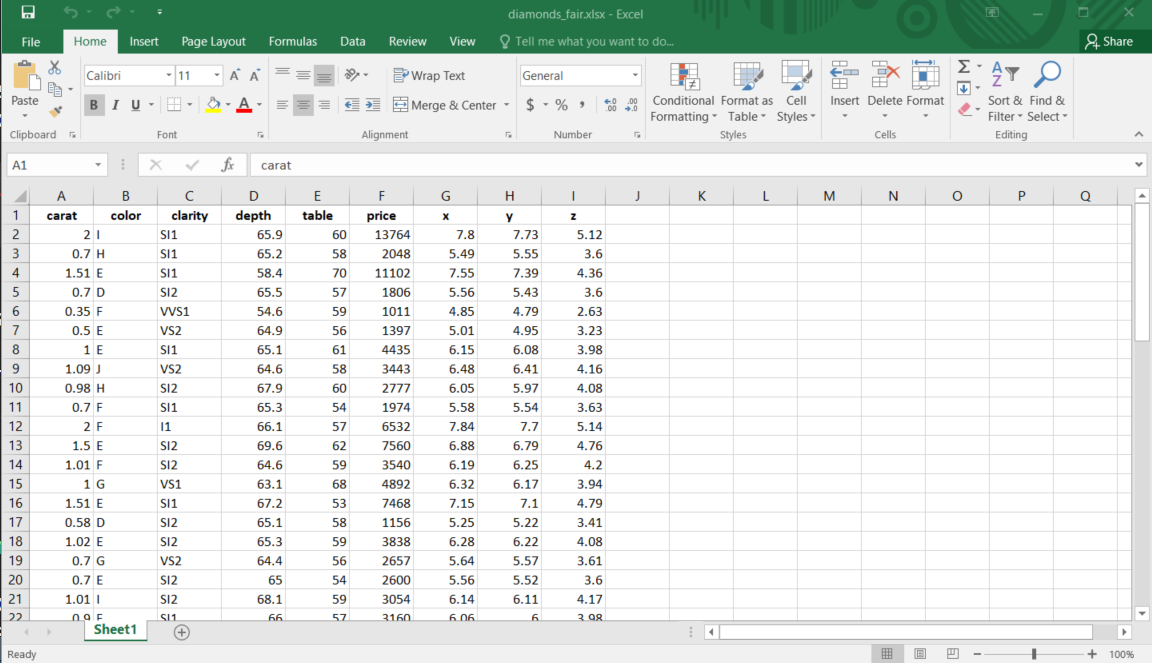
After processing your Excel data in R, you may wish to export the cleaned data. The write_xlsx() function from the writexl package enables you to save your data frame as a new Excel file:

write_xlsx(diamonds_fair, path = "r-data/diamonds_fair.xlsx")

Figure 4.11 shows the resulting Excel file. By default, column names are included and bolded. You can disable these features by setting the col_names and format_headers arguments to FALSE.

Figure 4.11: Spreadsheet View of the File diamond-fair.xlsx in Excel.

4.8.3 Labelled Data

Labelled data commonly originates from specialised statistical software such as SPSS, Stata, or SAS. These datasets often include value labels that describe the meaning of each code. R can import these files using the haven package. Like the readxl, haven is not part of the core tidyverse, but is installed automatically with it; however, you must load it explicitly.

For example:

• SPSS

  • read_sav(): This function imports data from SPSS files (files with .sav extension) into R.

  • write_sav(): Exports a data frame from R back to SPSS format.

• Stata

  • read_dta(): For Stata users, this function imports Stata files into R.

  • write_dta(): Similarly, this function lets you export data frames to Stata format.

• SAS

  • read_sas() reads .sas7bdat + .sas7bcat files and read_xpt() reads SAS transport files (versions 5 and 8).

  • write_xpt() writes SAS transport files (versions 5 and 8).

Example 1: Reading an SPSS File

Suppose you have an SPSS file named wages.sav. You can import it using haven as follows:

library(tidyverse)
library(haven)

wages <- read_sav("r-data/wages.sav")

wages

#> # A tibble: 400 × 9
#>       id  educ south                 sex     exper  wage occup   marr    ed     
#>    <dbl> <dbl> <dbl+lbl>             <dbl+l> <dbl> <dbl> <dbl+l> <dbl+l> <dbl+l>
#>  1     3    12 0 [does not live in … 0 [Mal…    17  7.5  6 [Oth… 1 [Mar… 2 [Hig…
#>  2     4    13 0 [does not live in … 0 [Mal…     9 13.1  6 [Oth… 0 [Not… 3 [Som…
#>  3     5    10 1 [lives in South]    0 [Mal…    27  4.45 6 [Oth… 0 [Not… 1 [Les…
#>  4    12     9 1 [lives in South]    0 [Mal…    30  6.25 6 [Oth… 0 [Not… 1 [Les…
#>  5    13     9 1 [lives in South]    0 [Mal…    29 20.0  6 [Oth… 1 [Mar… 1 [Les…
#>  6    14    12 0 [does not live in … 0 [Mal…    37  7.3  6 [Oth… 1 [Mar… 2 [Hig…
#>  7    17    11 0 [does not live in … 0 [Mal…    16  3.65 6 [Oth… 0 [Not… 1 [Les…
#>  8    20    12 0 [does not live in … 0 [Mal…     9  3.75 6 [Oth… 0 [Not… 2 [Hig…
#>  9    21    11 1 [lives in South]    0 [Mal…    14  4.5  6 [Oth… 1 [Mar… 1 [Les…
#> 10    23     6 1 [lives in South]    0 [Mal…    45  5.75 6 [Oth… 1 [Mar… 1 [Les…
#> # ℹ 390 more rows

In some cases, haven’s read_sav() may not fully process labelled variables. In such instances, you can use the bulkreadr package for a more seamless import:

library(bulkreadr)

# Import SPSS data with automatic label conversion

wages_data <- read_spss_data("r-data/wages.sav")

wages_data

#> # A tibble: 400 × 9
#>       id  educ south                  sex   exper  wage occup marr        ed    
#>    <dbl> <dbl> <fct>                  <fct> <dbl> <dbl> <fct> <fct>       <fct> 
#>  1     3    12 does not live in South Male     17  7.5  Other Married     High …
#>  2     4    13 does not live in South Male      9 13.1  Other Not married Some …
#>  3     5    10 lives in South         Male     27  4.45 Other Not married Less …
#>  4    12     9 lives in South         Male     30  6.25 Other Not married Less …
#>  5    13     9 lives in South         Male     29 20.0  Other Married     Less …
#>  6    14    12 does not live in South Male     37  7.3  Other Married     High …
#>  7    17    11 does not live in South Male     16  3.65 Other Not married Less …
#>  8    20    12 does not live in South Male      9  3.75 Other Not married High …
#>  9    21    11 lives in South         Male     14  4.5  Other Married     Less …
#> 10    23     6 lives in South         Male     45  5.75 Other Married     Less …
#> # ℹ 390 more rows

Example 2: Writing to a SPSS File

After performing analyses or modifications on your SPSS data, you may wish to export the results back to an SPSS file:

wages_data |> write_sav("wages.sav")

Example 3: Reading Stata File

Similarly, if you have a Stata dataset (for example, automobile.dta), you can import it using bulkreadr:

# Import Stata data with bulkreadr

automobile <- read_stata_data("r-data/automobile.dta")

glimpse(automobile)

#> Rows: 32
#> Columns: 11
#> $ mpg  <dbl> 21.0, 21.0, 22.8, 21.4, 18.7, 18.1, 14.3, 24.4, 22.8, 19.2, 17.8,…
#> $ cyl  <dbl> 6, 6, 4, 6, 8, 6, 8, 4, 4, 6, 6, 8, 8, 8, 8, 8, 8, 4, 4, 4, 4, 8,…
#> $ disp <dbl> 160.0, 160.0, 108.0, 258.0, 360.0, 225.0, 360.0, 146.7, 140.8, 16…
#> $ hp   <dbl> 110, 110, 93, 110, 175, 105, 245, 62, 95, 123, 123, 180, 180, 180…
#> $ drat <dbl> 3.90, 3.90, 3.85, 3.08, 3.15, 2.76, 3.21, 3.69, 3.92, 3.92, 3.92,…
#> $ wt   <dbl> 2.620, 2.875, 2.320, 3.215, 3.440, 3.460, 3.570, 3.190, 3.150, 3.…
#> $ qsec <dbl> 16.46, 17.02, 18.61, 19.44, 17.02, 20.22, 15.84, 20.00, 22.90, 18…
#> $ vs   <dbl> 0, 0, 1, 1, 0, 1, 0, 1, 1, 1, 1, 0, 0, 0, 0, 0, 0, 1, 1, 1, 1, 0,…
#> $ am   <dbl> 1, 1, 1, 0, 0, 0, 0, 0, 0, 0, 0, 0, 0, 0, 0, 0, 0, 1, 1, 1, 0, 0,…
#> $ gear <dbl> 4, 4, 4, 3, 3, 3, 3, 4, 4, 4, 4, 3, 3, 3, 3, 3, 3, 4, 4, 4, 3, 3,…
#> $ carb <dbl> 4, 4, 1, 1, 2, 1, 4, 2, 2, 4, 4, 3, 3, 3, 4, 4, 4, 1, 2, 1, 1, 2,…

Example 4: Writing to a Stata File

If you wish to export a data frame to a Stata format, you can use haven’s write function:

automobile |> write_dta("automobile-data.dta")

The rio Package

The rio package complements other data-importing packages by providing a one-stop solution for data import and export in R. It handles a wide variety of file types—CSV, Excel, SPSS, Stata, and more—so you don’t need to remember different functions for each format.

• import(): Automatically detects the file type and imports your data into R, simplifying the process of reading data from diverse sources.

• export(): Export your data frame to various file formats with ease, whether you are creating a CSV file, an Excel workbook, or a file for statistical software.

For further details on the extensive capabilities of the rio package, please refer to the rio documentation.

Example 1: Data Import with rio Package

In this example, we load the telco-customer-churn.csv file from the r-data folder using the import() function. This function automatically detects the file type and loads the data accordingly.

library(rio)

# Import data from a CSV file
telco_customer_churn <- import("r-data/telco-customer-churn.csv")

After importing the data, you may wish to perform some basic cleaning. For instance, you might standardise variable names using the clean_names() function from the janitor package:

library(janitor)

# Clean variable names
telco_customer_churn <- telco_customer_churn |>
  clean_names()

# Glimpse the structure of the data
telco_customer_churn |>
  glimpse()

#> Rows: 7,043
#> Columns: 21
#> $ customer_id       <chr> "7590-VHVEG", "5575-GNVDE", "3668-QPYBK", "7795-CFOC…
#> $ gender            <chr> "Female", "Male", "Male", "Male", "Female", "Female"…
#> $ senior_citizen    <int> 0, 0, 0, 0, 0, 0, 0, 0, 0, 0, 0, 0, 0, 0, 0, 0, 0, 0…
#> $ partner           <chr> "Yes", "No", "No", "No", "No", "No", "No", "No", "Ye…
#> $ dependents        <chr> "No", "No", "No", "No", "No", "No", "Yes", "No", "No…
#> $ tenure            <int> 1, 34, 2, 45, 2, 8, 22, 10, 28, 62, 13, 16, 58, 49, …
#> $ phone_service     <chr> "No", "Yes", "Yes", "No", "Yes", "Yes", "Yes", "No",…
#> $ multiple_lines    <chr> "No phone service", "No", "No", "No phone service", …
#> $ internet_service  <chr> "DSL", "DSL", "DSL", "DSL", "Fiber optic", "Fiber op…
#> $ online_security   <chr> "No", "Yes", "Yes", "Yes", "No", "No", "No", "Yes", …
#> $ online_backup     <chr> "Yes", "No", "Yes", "No", "No", "No", "Yes", "No", "…
#> $ device_protection <chr> "No", "Yes", "No", "Yes", "No", "Yes", "No", "No", "…
#> $ tech_support      <chr> "No", "No", "No", "Yes", "No", "No", "No", "No", "Ye…
#> $ streaming_tv      <chr> "No", "No", "No", "No", "No", "Yes", "Yes", "No", "Y…
#> $ streaming_movies  <chr> "No", "No", "No", "No", "No", "Yes", "No", "No", "Ye…
#> $ contract          <chr> "Month-to-month", "One year", "Month-to-month", "One…
#> $ paperless_billing <chr> "Yes", "No", "Yes", "No", "Yes", "Yes", "Yes", "No",…
#> $ payment_method    <chr> "Electronic check", "Mailed check", "Mailed check", …
#> $ monthly_charges   <dbl> 29.85, 56.95, 53.85, 42.30, 70.70, 99.65, 89.10, 29.…
#> $ total_charges     <dbl> 29.85, 1889.50, 108.15, 1840.75, 151.65, 820.50, 194…
#> $ churn             <chr> "No", "No", "Yes", "No", "Yes", "Yes", "No", "No", "…

Example 2: Exporting Data with rio Package

After importing your data, it is often necessary to review and adjust variable types. In this example, all character columns (which represent categorical variables) are converted to factors, except for the customer_id column which remains as a character to preserve its unique identifier status. Once the data is transformed (see Chapter 5 for further discussion on data transformation), we filter the data to include only records where dependents is "Yes" and then export the result to an Excel file.

telco_customer_churn <- telco_customer_churn %>%
  mutate(across(where(is.character), as.factor)) %>%
  mutate(customer_id = as.character(customer_id))

# Filter data and export to an Excel file
telco_customer_churn |>
  filter(dependents == "Yes") |>
  export("telco_customer_churn.xlsx")

In this manner, rio offers a streamlined process for both importing and exporting data, reducing the need to juggle multiple packages or recall numerous functions.

4.8.4 Web Scraping

Web scraping is the process of extracting data from websites, and R provides several tools to facilitate this task. The ralger package is one such tool, offering a streamlined approach to retrieving and parsing data from web pages. Whether you are collecting data for text analysis, monitoring website updates, or simply gathering information from the web, ralger simplifies the process.

4.8.4.1 Key Features of the ralger Package

• Simplified Data Retrieval: ralger allows you to quickly download the HTML content of a web page without requiring multiple packages.

• CSS Selector Support: The package enables you to extract specific elements from a webpage by utilising CSS selectors.

• Integrated Parsing Functions: Once the HTML is retrieved, ralger provides functions to parse and manipulate the data efficiently.

Example 1: Extracting a Non-Table HTML Data

When web content is provided in HTML format, you can use the tidy_scrap() function from the ralger package to extract data into a tidy data frame. This function returns a data frame based on the arguments you supply. The key arguments are:

• link: The URL of the website you wish to scrape.

• nodes: A vector of CSS selectors corresponding to the HTML elements you want to extract. These elements will form the columns of your data frame.

• colnames: A vector of names to assign to the columns, which should match the order of the selectors specified in the nodes argument.

• clean: If set to TRUE, the function will clean the tibble’s columns.

• askRobot: If enabled, the function will consult the site’s robots.txt file to verify whether scraping is permitted.

In this example, we will scrape the Hacker News website (https://news.ycombinator.com). We aim to extract a tidy data frame containing the following elements:

• The story title.

• The site name (if available).

• The score of the story.

• Additional subline information.

• The username of the poster.

Here is how you can achieve this using the tidy_scrap() function with improved column names:

library(ralger)

# Define the URL for Hacker News
url <- "https://news.ycombinator.com/"

# Define the CSS selectors for the elements to extract
nodes <- c(".titleline > a", ".sitestr", ".score", ".subline a+ a", ".hnuser")

# Define descriptive column names for the resulting data frame
colnames <- c("title", "site", "score", "subline", "username")

# Extract the data from all pages using tidy_scrap()
news_data <- tidy_scrap(
  link = url,
  nodes = nodes,
  colnames = colnames,
  clean = TRUE
)

#> Warning in (function (..., deparse.level = 1) : number of rows of result is not
#> a multiple of vector length (arg 3)

news_data

#> # A tibble: 30 × 5
#>    title                                            site  score subline username
#>    <chr>                                            <chr> <chr> <chr>   <chr>   
#>  1 Archival Storage                                 dshr… 142 … 75 com… rbanffy 
#>  2 Show HN: OpenTimes – Free travel times between … open… 59 p… 19 com… dfsnow  
#>  3 The High Heel Problem                            simo… 45 p… 5 comm… lehi    
#>  4 Deep Learning Is Not So Mysterious or Different  arxi… 218 … 56 com… wuubuu  
#>  5 Hidden Messages in Emojis and Hacking the US Tr… slam… 62 p… 26 com… nickagl…
#>  6 Alphabet spins out Taara – Internet over lasers  x.co… 80 p… 86 com… tadeegan
#>  7 PrintedLabs – 3D printable optical experiment e… uni-… 9 po… discuss aethert…
#>  8 HTTP/3 is everywhere but nowhere                 http… 281 … 283 co… doener  
#>  9 Luthor (YC F24) Is Hiring Ruby on Rails Enginee… ycom… 8 po… discuss ftr1200 
#> 10 Show HN: Cascii – A portable ASCII diagram buil… gith… 829 … 325 co… radeeya…
#> # ℹ 20 more rows

Tip

In this code:

• The tidy_scrap() function is called with the Hacker News URL.

• The nodes argument specifies the CSS selectors for the elements we wish to extract. The nodes vector contains the CSS selectors:

  • “.titleline > a”: extracts the story title,

  • “.sitestr”: extracts the site name,

  • “.score”: extracts the story score,

  • “.subline a+ a”: extracts additional subline information,

  • “.hnuser”: extracts the username.

• The colnames argument assigns clear and descriptive names to the columns—namely "title", "site", "score", "subline", and "username".

• The function returns a tidy data frame in which all columns are of character class; you may convert these to other types as required for your analysis.

If you wish to scrape multiple list pages, you can use tidy_scrap() in conjunction with paste0(). Suppose you want to scrape pages 1 through 5 of Hacker News:

# Define the URL for Hacker News
url <- "https://news.ycombinator.com/"

# Create a vector of URLs for pages 1 to 5
links <- paste0(url, "?p=", seq(1, 5, 1))

# Extract the data from all pages using tidy_scrap()
news_data <- tidy_scrap(
  link = links,
  nodes = nodes,
  colnames = colnames
)

#> Undefined Error: Error in open.connection(x, "rb"): Could not resolve host: news.ycombinator.com

#> Warning in (function (..., deparse.level = 1) : number of rows of result is not
#> a multiple of vector length (arg 2)

news_data

#> # A tibble: 150 × 5
#>    title                                            site  score subline username
#>    <chr>                                            <chr> <chr> <chr>   <chr>   
#>  1 Archival Storage                                 dshr… <NA>  75 com… rbanffy 
#>  2 Show HN: OpenTimes – Free travel times between … open… <NA>  19 com… dfsnow  
#>  3 The High Heel Problem                            simo… <NA>  5 comm… lehi    
#>  4 Deep Learning Is Not So Mysterious or Different  arxi… <NA>  56 com… wuubuu  
#>  5 Hidden Messages in Emojis and Hacking the US Tr… slam… <NA>  26 com… nickagl…
#>  6 Alphabet spins out Taara – Internet over lasers  x.co… <NA>  86 com… tadeegan
#>  7 PrintedLabs – 3D printable optical experiment e… uni-… <NA>  discuss aethert…
#>  8 HTTP/3 is everywhere but nowhere                 http… <NA>  283 co… doener  
#>  9 Luthor (YC F24) Is Hiring Ruby on Rails Enginee… ycom… <NA>  discuss ftr1200 
#> 10 Show HN: Cascii – A portable ASCII diagram buil… gith… <NA>  325 co… radeeya…
#> # ℹ 140 more rows

Note

Since Hacker News is a dynamic website, the content may change over time. Therefore, if you rerun the same lines of code at a later time, the extracted results may differ from those obtained previously.

Example 2: Extracting an HTML Table

The ralger package also includes a function called table_scrap() for extracting HTML tables from a web page. Suppose you want to extract an HTML table from a page listing the highest lifetime gross revenues in the cinema industry. You can use the following code:

# Extract an HTML table from the specified URL

url <- "https://www.boxofficemojo.com/chart/top_lifetime_gross/?area=XWW"

lifetime_gross <- table_scrap(link = url)

#> Warning: The `fill` argument of `html_table()` is deprecated as of rvest 1.0.0.
#> ℹ An improved algorithm fills by default so it is no longer needed.
#> ℹ The deprecated feature was likely used in the rvest package.
#>   Please report the issue at <https://github.com/tidyverse/rvest/issues>.

# Display the extracted table
lifetime_gross

#> # A tibble: 200 × 4
#>     Rank Title                                      `Lifetime Gross`  Year
#>    <int> <chr>                                      <chr>            <int>
#>  1     1 Avatar                                     $2,923,710,708    2009
#>  2     2 Avengers: Endgame                          $2,799,439,100    2019
#>  3     3 Avatar: The Way of Water                   $2,320,250,281    2022
#>  4     4 Titanic                                    $2,264,812,968    1997
#>  5     5 Ne Zha 2                                   $2,084,181,921    2025
#>  6     6 Star Wars: Episode VII - The Force Awakens $2,071,310,218    2015
#>  7     7 Avengers: Infinity War                     $2,052,415,039    2018
#>  8     8 Spider-Man: No Way Home                    $1,952,732,181    2021
#>  9     9 Inside Out 2                               $1,698,863,816    2024
#> 10    10 Jurassic World                             $1,671,537,444    2015
#> # ℹ 190 more rows

Note

If you are dealing with a web page that contains multiple HTML tables, you can use the choose argument with table_scrap() to target a specific table. For more advanced use cases and customisation options, please refer to the package documentation.

By incorporating web scraping into your data analysis workflow, you can dynamically collect data from the web and integrate it with your existing analyses, thereby broadening the scope of your data-driven insights.

4.8.5 Bringing It All Together

When working on a project, it is best practice to organise your data and code within a dedicated RStudio project. Store your data files (be they flat files, spreadsheets, or labelled files) in a folder (for example, data/), and use relative paths when reading and writing data. This approach promotes reproducibility and clarity. Let us now practise importing data using the gapminder.csv file.

Before We Begin:

1. Create a Directory
   Create a new folder on your desktop called Experiment 4.3.

2. Download Data
   Visit Google Drive to download the r-data folder (refer to Appendix B.1 for additional information). Once downloaded, unzip the folder and move it into your Experiment 4.3 folder.

3. Create an RStudio Project
   Open RStudio and set up a new project as follows:

   • Go to File > New Project.
     
   • Select Existing Directory and navigate to your Experiment 4.3 folder.
     This project setup will organise your work and ensure that everything related to this experiment is contained in one place.

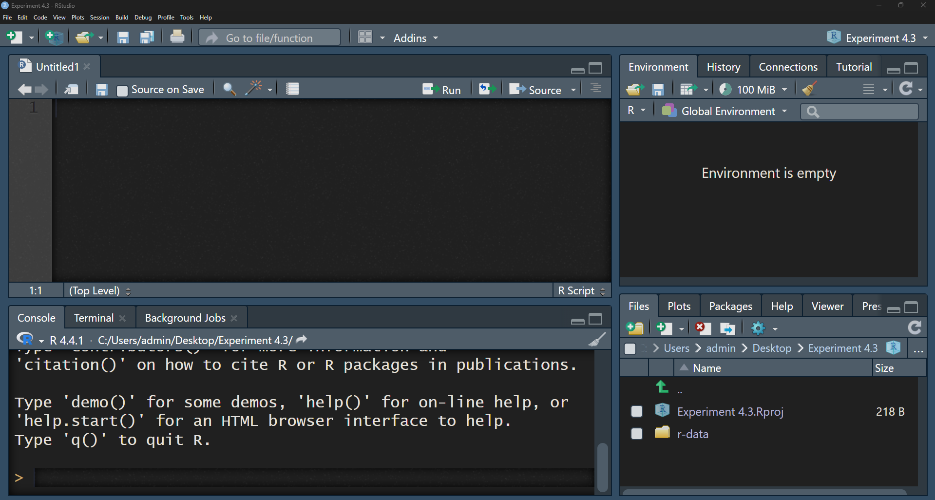
Your project structure should resemble the one shown in Figure 4.12:

Figure 4.12: Starting a New R Project in RStudio

Now, let us import the gapminder.csv file from the r-data folder into R using the tidyverse package for convenient data manipulation and visualisation:

library(tidyverse)

# Load the gapminder data
gapminder <- read_csv("r-data/gapminder.csv")

#> Rows: 1704 Columns: 6
#> ── Column specification ────────────────────────────────────────────────────────
#> Delimiter: ","
#> chr (2): country, continent
#> dbl (4): year, lifeExp, pop, gdpPercap
#> 
#> ℹ Use `spec()` to retrieve the full column specification for this data.
#> ℹ Specify the column types or set `show_col_types = FALSE` to quiet this message.

# Explore the data
names(gapminder)

#> [1] "country"   "continent" "year"      "lifeExp"   "pop"       "gdpPercap"

dim(gapminder)

#> [1] 1704    6

head(gapminder)

#> # A tibble: 6 × 6
#>   country     continent  year lifeExp      pop gdpPercap
#>   <chr>       <chr>     <dbl>   <dbl>    <dbl>     <dbl>
#> 1 Afghanistan Asia       1952    28.8  8425333      779.
#> 2 Afghanistan Asia       1957    30.3  9240934      821.
#> 3 Afghanistan Asia       1962    32.0 10267083      853.
#> 4 Afghanistan Asia       1967    34.0 11537966      836.
#> 5 Afghanistan Asia       1972    36.1 13079460      740.
#> 6 Afghanistan Asia       1977    38.4 14880372      786.

summary(gapminder)

#>    country           continent              year         lifeExp     
#>  Length:1704        Length:1704        Min.   :1952   Min.   :23.60  
#>  Class :character   Class :character   1st Qu.:1966   1st Qu.:48.20  
#>  Mode  :character   Mode  :character   Median :1980   Median :60.71  
#>                                        Mean   :1980   Mean   :59.47  
#>                                        3rd Qu.:1993   3rd Qu.:70.85  
#>                                        Max.   :2007   Max.   :82.60  
#>       pop              gdpPercap       
#>  Min.   :6.001e+04   Min.   :   241.2  
#>  1st Qu.:2.794e+06   1st Qu.:  1202.1  
#>  Median :7.024e+06   Median :  3531.8  
#>  Mean   :2.960e+07   Mean   :  7215.3  
#>  3rd Qu.:1.959e+07   3rd Qu.:  9325.5  
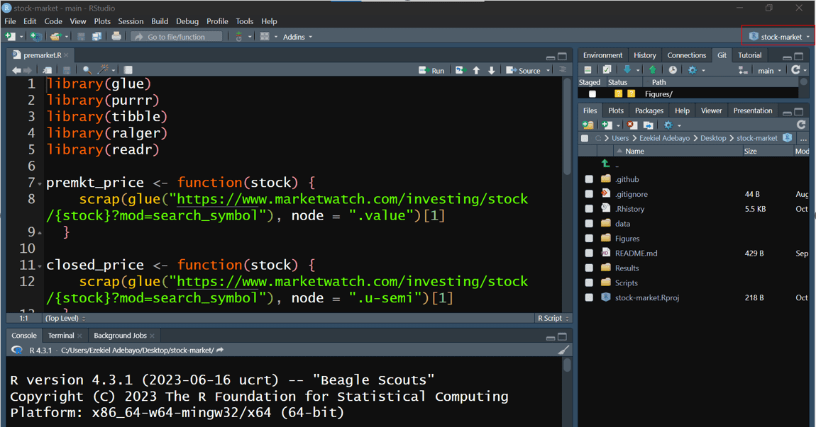
#>  Max.   :1.319e+09   Max.   :113523.1

After running this script, your dataset should be loaded into RStudio and ready for exploration. Your script should resemble the one in Figure 4.13:

Figure 4.13: Loading and Exploring Data in RStudio

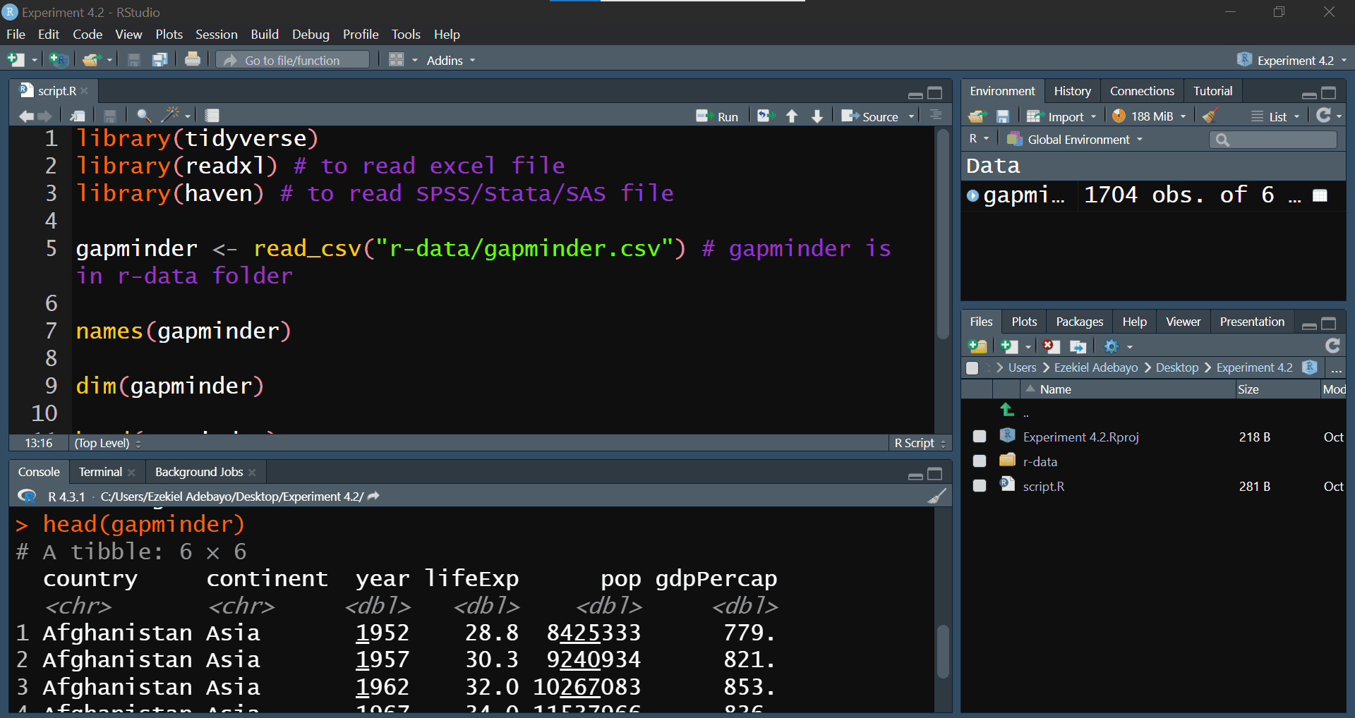
This setup ensures that everything required for your analysis is neatly organised, reproducible, and ready for you to begin analysing the gapminder data in R.

4.8.6 Practice Quiz 4.3

Question 1:

Which package is commonly used to read CSV files into R as tibbles?

1. readxl
   
2. haven
   
3. readr
   
4. writexl

Question 2:

If you need to import an Excel file, which function would you likely use?

1. read_csv()
   
2. read_xlsx()
   
3. read_sav()
   
4. read_dta()

Question 3:

Which package would you use to easily handle a wide variety of data formats without memorising specific functions for each?

1. rio
   
2. haven
   
3. janitor
   
4. readxl

Question 4:

After cleaning and analysing your data, which function would you use to write the results to a CSV file?

1. write_xlsx()
   
2. export()
   
3. write_csv()
   
4. import()

See the Solution to Quiz 4.3

4.8.7 Exercise 4.3.1: Medical Insurance Data

In this exercise, you’ll explore the medical-insurance.xlsx file located in the r-data folder. You can download this file from Google Drive. This dataset contains medical insurance information for various individuals. Below is an overview of each column:

1. User ID: A unique identifier for each individual.

2. Gender: The individual’s gender (‘Male’ or ‘Female’).

3. Age: The age of the individual in years.

4. AgeGroup: The age bracket the individual falls into.

5. Estimated Salary: An estimate of the individual’s yearly salary.

6. Purchased: Indicates whether the individual has purchased medical insurance (1 for Yes, 0 for No).

Your Tasks:

1. Importing and Basic Handling:

   • Create a new script and import the data from the Excel file.
   • How would you import this data if it’s in SPSS format?
   • Use the clean_names() function from the janitor package to make variable names consistent and easy to work with.
   • Can you display the first three rows of the dataset?
   • How many rows and columns does the dataset have?

2. Understanding the Data:

   • What are the column names in the dataset?
   • Can you identify the data types of each column?

3. Basic Descriptive Statistics:

   • What is the average age of the individuals in the dataset?
   • What’s the range of the estimated salaries?

4.9 Reflective Summary

In Lab 4, you have acquired essential skills to enhance your efficiency and effectiveness as an R programmer:

• Installing and Loading Packages: You learned how to find, install, and load packages from CRAN and external repositories like GitHub.

• Reproducible Workflows with RStudio Projects: You discovered the importance of organizing your work within RStudio Projects.

• Importing and Exporting Data: You practiced importing and exporting data in various formats (CSV, Excel, SPSS) using packages like readr, readxl, and haven.

These skills are fundamental for efficient data analysis, helping you manage diverse data sources, maintain integrity in your analyses, and collaborate more effectively. Congratulations on progressing as an R programmer and data analyst!

What’s Next?

In the next lab, we’ll delve into data transformation where will reshape raw data into a more useful format for data analysis.

---

1. It is common for a package to print out messages when you load it. These messages often include information about the package version, attached packages, or important notes from the authors. For example, when you load the tidyverse package. If you prefer to suppress these messages, you can use the suppressMessages() function: suppressMessages(library(tidyverse))

2. If you or your collaborators rely on spreadsheets to organise data, we highly recommend the paper “Data Organization in Spreadsheets” by Karl Broman and Kara Woo: https://doi.org/10.1080/00031305.2017.1375989. It provides valuable guidance on best practices and efficient data structuring techniques.

3. A tibble is a modern version of an R data frame that provides cleaner printing and more consistent behavior, especially within the tidyverse ecosystem.