3  Writing Custom Function

3.1 Introduction

Welcome to Lab 3! In this lab, we’ll explore how to write your own functions in R. Functions are essential in programming because they allow you to encapsulate code that performs specific tasks. This makes your programs more modular, readable, and easier to maintain. By designing custom functions, you can automate repetitive tasks, streamline your data analysis processes, and enhance the efficiency of your code.

3.2 Learning Objectives

By the end of this lab, you will be able to:

• Understand the Syntax of Functions in R
  Learn how to define functions using the function() keyword, specify arguments, and structure the function body to perform desired operations.

• Create Custom Functions
  Write your own functions to perform specific data analysis tasks, allowing you to reuse code and avoid repetition.

• Utilize Functions to Modularize and Streamline Code
  Break down complex data analysis tasks into smaller, manageable functions to make your code more organized and maintainable.

• Understand Variable Scope Within Functions
  Grasp how variable scope works in R, distinguishing between local and global variables, and understand how this affects the behaviour of your functions.

• Apply Best Practices in Function Design
  Implement best practices such as choosing meaningful function names, including documentation with comments, handling inputs and outputs effectively, and incorporating error handling.

• Demonstrate Understanding Through Practical Application
  Use the functions you create in real data analysis scenarios to show how they can simplify tasks and improve code efficiency.

By completing this lab, you’ll enhance your programming skills in R, enabling you to write code that is not only effective but also clean, reusable, and easy to understand. These skills are fundamental for any data analysis or data science work you’ll undertake in the future.

3.3 Prerequisites

Before starting this lab, you should have:

• Completed Lab 2 or have a basic understanding of R’s data structures (vectors, matrices, data frames, and lists).

• Familiarity with basic programming concepts (variables, loops, conditionals).

• An interest in learning how to enhance your R programming skills through custom functions.

3.4 Experiment 3.1: Understanding Functions in R

A function is a block of code designed to perform a specific task. Functions usually take in some form of data structure—like a value, vector, or dataframe—as arguments, process it, and return a result. R has many built-in functions like mean(), sum(), and plot(), but creating your own functions allows you to tailor operations to your specific needs. For instance, imagine you often perform repetitive data transformations, cleaning, or statistical analysis. Writing custom functions allows you to automate these tasks, saving time and reducing potential errors.

Figure 3.1: Core Functions in R Programming

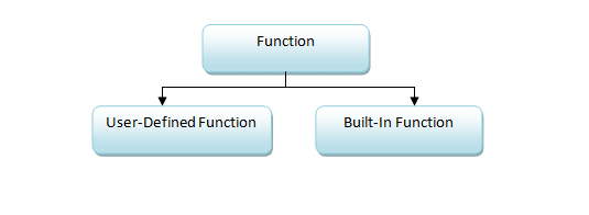
3.4.1 Types of Functions

Functions can be broadly categorized into two types:

Figure 3.2: Types of Functions in R Programming

• Built-in Functions: These are predefined functions provided by R, e.g., mean(), print().

• User-defined Functions: These are functions created by the user to perform specific tasks.

3.4.2 Why Write Your Own Function?

Creating your own functions has several advantages:

• Code Reusability: Functions promote code reuse and help you avoid repetition.

• Improved Readability: They make your code more readable and maintainable.

• Modular Programming: Functions allow for modular programming, where you can break down complex tasks into smaller, manageable pieces.

3.4.3 When Should You Write a Function?

Consider writing a function when:

• You find yourself repeating code.

• You need to perform a complex calculation multiple times.

• You want to make your code more organized and maintainable.

3.4.4 Creating Custom Function

A function in R has three main components:

• Function Name: A descriptive name that reflects the function’s purpose.

• Function Arguments: Inputs that the function will process. This could be any type of object—such as a scalar, matrix, dataframe, vector, or logical.

• Function Body: The code that defines what the function does.

The general structure of a function is:

#|

function_name <- function(arg1, arg2, ...) {
  # Function body
  # ...
  return(result)
}

Best Practice

• Naming Conventions: Use snake_case and descriptive names.

• Comments: Include comments to explain complex logic.

• Indentation: Use consistent indentation for readability.

If you create an object inside a function that you want to use outside of it, you need to return it using the return() function.

3.4.4.1 Calling a User-defined Function in R

You can call a user-defined function just like any built-in function, using its name. If the function accepts parameters or arguments, you pass them when calling the function.

3.4.5 Example 1: Squaring a Number

Let’s start by creating a simple function to square a number. This example will introduce you to defining and using functions in R.

Defining the Function:

First, we’ll define the function square_it. This function will take a single input, x, and return its square. Here’s how you would write it:

# Function to square a number
square_it <- function(x) {
  result <- x^2
  return(result)
}

Now, whenever you call square_it() with a numerical input, it will output the square of that number.

Testing the Function

To verify that the function works as expected, try squaring a few numbers:

• Test with 12:

square_it(12)

#> [1] 144

• Test with vector, product_prices:

product_prices <- c(19.99, 5.49, 12.89, 99.99, 49.95)

square_it(product_prices)

#> [1]  399.6001   30.1401  166.1521 9998.0001 2495.0025

Reflection Question

• Why is it beneficial to write a function for squaring a number instead of writing x^2 each time?

3.4.6 Example 2: Checking for Missing Values

Next, let’s create a function that checks for missing values in a dataset and counts them.

Defining the Function

We’ll define a function called check_NA as follows:

# Function to check for missing values
check_NA <- function(data) {
  any_na <- anyNA(data)
  na_count <- sum(is.na(data))
  announcement <- paste("Any NA:", any_na, "| Total NA:", na_count)
  return(announcement)
}

Testing the Function

You can use this function to check for missing values in various datasets.

• For the airquality dataset:

check_NA(airquality)

#> [1] "Any NA: TRUE | Total NA: 44"

• For the iris dataset:

check_NA(iris)

#> [1] "Any NA: FALSE | Total NA: 0"

Running these commands will let you know if there are any missing values in the dataset and provide the total count of missing values.

3.5 Experiment 3.2: Advanced Function Examples

3.5.1 Example 3: Calculating the Statistical Mode

There is no built-in function in R to calculate the mode, so let’s create one.

statistical_mode <- function(x) {
  # Get unique values
  uniqx <- unique(x)

  # Count frequencies of each unique value
  freq <- tabulate(match(x, uniqx))

  # Find the maximum frequency
  max_freq <- max(freq)

  # Find all values with the maximum frequency
  modes <- uniqx[freq == max_freq]

  # Handle cases
  if (length(modes) == length(uniqx)) {
    return("No mode: All values occur with equal frequency.")
  } else if (length(modes) > 1) {
    return(list("Multiple Modes" = modes, "Frequency" = max_freq))
  } else {
    return(list("Mode" = modes, "Frequency" = max_freq))
  }
}

Explanation

1. Unique Values:
   • unique(x) extracts distinct values from the input vector.
2. Frequency Count:
   • tabulate(match(x, uniqx)) counts occurrences of each unique value.
3. Maximum Frequency:
   • max(freq) identifies the highest frequency.
4. Multiple Modes:
   • The function checks if more than one value has the maximum frequency.
5. No Mode:
   • If all unique values occur equally, the function returns a message stating there is no mode.

This statistical_mode() function will handle every possible scenario, including:

1. Single Mode: Returns the value with the highest frequency.

2. Multiple Modes: Returns all values with the highest frequency.

3. No Mode: Returns a message if all values appear with equal frequency (no distinct mode).

Testing the Function

• Test 1: Single Mode

  calls <- c(
    0, 2, 6, 2, 2, 0, 0, 1, 1, 5, 3, 1, 0,
    2, 3, 1, 2, 1, 4, 4, 5, 0, 5, 1, 2, 2,
    2, 0, 4, 0, 6
  )
  
  statistical_mode(calls)

  #> $Mode
  #> [1] 2
  #> 
  #> $Frequency
  #> [1] 8

• Test 2: Multiple Modes

  scores <- c(5, 5, 6, 6, 7, 8)
  
  statistical_mode(scores)

  #> $`Multiple Modes`
  #> [1] 5 6
  #> 
  #> $Frequency
  #> [1] 2

• Test 3: No Mode

  values <- c(1, 2, 3, 4, 5)
  
  statistical_mode(values)

  #> [1] "No mode: All values occur with equal frequency."

3.5.2 Example 4: Data Frame Operation Using switch()

Suppose we have employee data and want to perform various operations based on user input. The available operations are:

• “summary”: Get a summary of the data frame.

• “add_column”: Add a new column to the data frame.

• “filter”: Filter the data frame based on a specified condition.

• “group_stats”: Calculate group-wise statistics.

To follow along with this example, please refer to Chapter 1.8.5 for a detailed tutorial and comprehensive understanding of the switch() function.

Step 1: Creating a Sample Data Frame

#|
library(tidyverse)

# Sample employee data
staff_data <- data.frame(
  EmployeeID = 1:6,
  Name = c("Alice", "Ebunlomo", "Festus", "Othniel", "Bob", "Testimony"),
  Department = c("HR", "IT", "Finance", "Data Science", "Marketing", "Finance"),
  Salary = c(70000, 80000, 75000, 82000, 73000, 78000)
)

staff_data

#>   EmployeeID      Name   Department Salary
#> 1          1     Alice           HR  70000
#> 2          2  Ebunlomo           IT  80000
#> 3          3    Festus      Finance  75000
#> 4          4   Othniel Data Science  82000
#> 5          5       Bob    Marketing  73000
#> 6          6 Testimony      Finance  78000

Step 2: Defining the Function

# Define the function
data_frame_operation <- function(data, operation = "filter" # or any of "summary",
                                 #  "add_column", filter", "group_stats"
) {
  result <- switch(operation,

    # Case 1: Summary of the data frame
    summary = {
      print("Summary of Data Frame:")
      summary(data)
    },

    # Case 2: Add a new column 'Bonus' which is 10% of the Salary
    add_column = {
      data$Bonus <- data$Salary * 0.10
      print("Data Frame after adding 'Bonus' column:")
      data
    },

    # Case 3: Filter employees with Salary > 75,000
    filter = {
      filtered_data <- filter(data, Salary > 75000)
      print("Filtered Data Frame (Salary > 75,000):")
      filtered_data
    },

    # Case 4: Group-wise average salary
    group_stats = {
      group_summary <- data %>%
        group_by(Department) %>%
        summarize(Average_Salary = mean(Salary))
      print("Group-wise Average Salary:")
      group_summary
    },

    # Default case
    {
      print("Invalid operation. Please choose a valid option.")
      NULL
    }
  )

  # Return the result
  return(result)
}

Explanation:

• Function data_frame_operation:

  • Parameters:

    • data: The data frame to operate on.

    • operation: A string specifying the operation to perform.

  • Using switch():

    • Each case corresponds to a specific operation.

    • Cases that involve multiple expressions are wrapped in {}.

    • The last expression in the block is returned as the result of the case.

    • If no match is found, the final unnamed argument serves as the default case.

  • Operations:

    • “summary”: Provides a summary of the data frame.

    • “add_column”: Adds a new column Bonus (10% of Salary) to the data frame.

    • “filter”: Filters the data frame to include only employees with a salary greater than $75,000.

    • “group_stats”: Calculates the average salary for each department.

  • Default Case: Prints an error message and returns NULL if the operation is invalid.

  • Return Value: The result of the operation is returned by the function.

Step 3: Testing the Function

Let’s test the function with different operations.

Example 1: Summary of the Data Frame

# Perform the 'summary' operation
data_frame_operation(staff_data, "summary")

#> [1] "Summary of Data Frame:"

#>    EmployeeID       Name            Department            Salary     
#>  Min.   :1.00   Length:6           Length:6           Min.   :70000  
#>  1st Qu.:2.25   Class :character   Class :character   1st Qu.:73500  
#>  Median :3.50   Mode  :character   Mode  :character   Median :76500  
#>  Mean   :3.50                                         Mean   :76333  
#>  3rd Qu.:4.75                                         3rd Qu.:79500  
#>  Max.   :6.00                                         Max.   :82000

Example 2: Add a New Column

# Perform the 'add_column' operation
data_frame_operation(staff_data, "add_column")

#> [1] "Data Frame after adding 'Bonus' column:"

#>   EmployeeID      Name   Department Salary Bonus
#> 1          1     Alice           HR  70000  7000
#> 2          2  Ebunlomo           IT  80000  8000
#> 3          3    Festus      Finance  75000  7500
#> 4          4   Othniel Data Science  82000  8200
#> 5          5       Bob    Marketing  73000  7300
#> 6          6 Testimony      Finance  78000  7800

Example 3: Filter the Data Frame

# Perform the 'filter' operation
data_frame_operation(staff_data, "filter")

#> [1] "Filtered Data Frame (Salary > 75,000):"

#>   EmployeeID      Name   Department Salary
#> 1          2  Ebunlomo           IT  80000
#> 2          4   Othniel Data Science  82000
#> 3          6 Testimony      Finance  78000

Example 4: Group-wise Statistics

# Perform the 'group_stats' operation
data_frame_operation(staff_data, "group_stats")

#> [1] "Group-wise Average Salary:"

#> # A tibble: 5 × 2
#>   Department   Average_Salary
#>   <chr>                 <dbl>
#> 1 Data Science          82000
#> 2 Finance               76500
#> 3 HR                    70000
#> 4 IT                    80000
#> 5 Marketing             73000

Example 5: Invalid Operation

# Attempt an invalid operation
data_frame_operation(staff_data, "view")

#> [1] "Invalid operation. Please choose a valid option."

#> NULL

Caution

Common Pitfall:

• Missing Libraries: Forgetting to load required packages like dplyr.

• Tip: Include library() calls within the function or check if the package is installed.

3.5.3 Exercise 3.1.1: Temperature Conversion

Now, it’s your turn to create a function.

Your Task: Create a function to convert Celsius (C) to Fahrenheit (F). You can use the formula:

\(\text{F} = \text{C} \times 1.8 + 32\)

Instructions:

1. Define the Function

   • Name the function celsius_to_fahrenheit.

   • It should take one argument, the temperature in Celsius.

2. Implement the Formula

   • Inside the function, apply the formula to convert Celsius to Fahrenheit.

3. Return the Result

   • The function should return the Fahrenheit temperature.

Test Your Function:

Use your function to convert the following Celsius temperatures to Fahrenheit:

• 100°C

• 75°C

• 120°C

For each temperature, call your function and verify that it returns the correct Fahrenheit value.

See the Solution to Exercise 3.1.1

3.5.4 Exercise 3.1.2: Pythagoras Theorem

Create a function to:

Your Task: Create a function called pythagoras to calculate the hypotenuse (c) of a right-angled triangle using Pythagoras’ theorem:

\[c = \sqrt{a^2 + b^2}\]

where a and b are the lengths of the other two sides.

Figure 3.3: Geometric Representation: Right-Angled Triangle

Instructions:

1. Define the Function

   • Name the function pythagoras.

   • It should take two arguments: a and b.

2. Implement the Formula

   • Inside the function, calculate the hypotenuse using the Pythagorean theorem.

3. Return the Result

   • The function should return the length of the hypotenuse.

Test Your Function:

Use your pythagoras function to calculate the hypotenuse for the following triangles:

• For \(a = 4.1\) and \(b = 2.6\)
• For \(a = 3\) and \(b = 4\)

Call your function with these values and verify that it returns the correct hypotenuse length.

See the Solution to Exercise 3.1.2

3.5.5 Exercise 3.1.3: Staff Data Manipulation Using switch()

Based on the example in Section 3.5.2, try modifying the code to include an additional operation:

• “raise_salary”: Increase the salary of all employees by 5%.

Instructions:

1. Add a new case to the switch() function for "raise_salary".

2. In this case, increase the Salary column by \(5\%\) and return the updated data frame.

3. Test the code by setting operation = "raise_salary".

Your Task:

# Modify the function to include 'raise_salary' operation
data_frame_operation <- function(..., operation) {
  result <- switch(operation,

    # Existing cases...

    # Case for 'raise_salary'
    raise_salary = {
      data$Salary <- data$Salary * ...
      print("Data Frame after 5% salary increase:")
      data
    },

    # Default case
    {
      print("Invalid operation. Please choose a valid option.")
      NULL
    }
  )

  # Return the result
  return(...)
}

Test the New Operation

# Perform the 'raise_salary' operation
data_frame_operation(staff_data, "---")

Replace the ... with the correct values and complete the exercise!

See the Solution to Exercise 3.1.3

Best Practices in Function Design

Meaningful Function Names

• Use descriptive names that convey the function’s purpose.

• Follow naming conventions (snake_case).

Handling Inputs and Outputs

• Validate input types and values.

• Provide clear and consistent return values.

Error Handling

• Use stop(), warning(), or message() to handle errors and warnings.

• Ensure that your function fails gracefully.

Example with Error Handling:

safe_divide <- function(a, b) {
  if (b == 0) {
    stop("Error: Division by zero is not allowed.")
  } else {
    return(a / b)
  }
}

# Testing the function
safe_divide(10, 2) # Returns 5

#> [1] 5

safe_divide(10, 0) # Error message

#> Error in safe_divide(10, 0): Error: Division by zero is not allowed.

Not validating inputs can lead to unexpected errors or incorrect results.

3.6 Experiment 3.3: Understanding Variable Scope

When writing a function, it’s crucial to understand how variables behave inside and outside the function. This concept is known as variable scope. Variable scope determines where a variable is accessible in your code and how changes to variables within the function can affect variables outside of them.

3.6.1 Local vs. Global Variables

• Local Variables: These are variables that are defined within a function. They exist only during the execution of that function and are not accessible outside of it.

• Global Variables: These are variables that are defined outside of any function. They exist in the global environment and can be accessed by any part of your script, including inside functions (unless shadowed by a local variable of the same name).

3.6.2 How Variable Scope Works in R

In R, each function has its own environment. This means that variables created inside a function (local variables) do not interfere with variables outside the function (global variables), even if they have the same name.

Example 1: Local Variable

Let’s look at an example to illustrate this:

variable_scope1 <- function() {
  local_var <- "I am a local variable!"
  print(local_var)
}

variable_scope1() # Prints "I am local"

#> [1] "I am a local variable!"

print(local_var) # Error: object 'local_var' not found

#> Error: object 'local_var' not found

In this example, local_var is a local variable within the variable_scope1() function. Trying to access local_var outside the function results in an error because it doesn’t exist in the global environment.

Example 2: Global Variable Access

Functions in R can access global variables unless there is a local variable with the same name:

global_var <- "I am global"

variable_scope2 <- function() {
  print(global_var)
}

variable_scope2() # Prints "I am global"

#> [1] "I am global"

Here, the function variable_scope2() accesses the global variable global_var because there is no local variable named global_var inside the function.

3.6.3 Variable Shadowing

When a local variable has the same name as a global variable, the local variable takes precedence within the function.

var <- "I am global"

variable_scope3 <- function() {
  var <- "I am local"
  print(var)
}

variable_scope3() # Prints "I am local"

#> [1] "I am local"

print(var) # Prints "I am global"

#> [1] "I am global"

In this case, the var variable inside variable_scope3() is local and doesn’t affect the global var variable.

Tip

Reflection Question:

• Why is it important to understand variable scope when writing functions?

Common Errors and Debugging Tips

• Syntax Errors: Check for missing commas, parentheses, or braces.

• Undefined Variables: Ensure all variables used in the function are defined.

• Incorrect Return Values: Make sure the function returns what you expect.

• Variable Scope Issues: Be mindful of local vs. global variables.

Debugging Tips:

• Use print() statements to check intermediate results.

• Use the debug() function to step through your function.

• Validate inputs at the start of your function.

3.6.4 Practice Quiz 3.1

Question 1:

What is the correct way to define a function in R?

1. function_name <- function { ... }

2. function_name <- function(...) { ... }

3. function_name <- function[ ... ] { ... }

4. function_name <- function(...) [ ... ]

Question 2:

A variable defined inside a function is accessible outside the function.

1. True

2. False

Question 3:

Which of the following is NOT a benefit of writing functions?

1. Code Reusability

2. Improved Readability

3. Increased Code Complexity

4. Modular Programming

See the Solution to Quiz 3.1

3.7 Summary

In this lab, you have developed essential skills in creating custom functions:

• Understanding the syntax of functions in R, including how to define functions using the function() keyword, specify arguments, and structure the function body.

• Creating and utilizing your own custom functions to perform specific data analysis tasks, promoting code reuse and avoiding repetition.

• Applying functions to modularize and streamline your code, breaking down complex tasks into smaller, manageable pieces for better organization and maintainability.

• Grasping variable scope within functions, distinguishing between local and global variables, and understanding how this affects the behavior of your functions.

• Implementing best practices in function design, such as choosing meaningful function names, including documentation with comments, handling inputs and outputs effectively, and incorporating error handling.

These skills are fundamental for efficient programming in R and will greatly enhance your data analysis capabilities. They form a strong foundation for more advanced topics you will encounter as you continue learning. Congratulations on advancing your programming expertise!

What’s Next?

In the next lab, we’ll delve into managing packages, creating reproducible workflows using RStudio project, and reading data from a file.