
2 Understanding Data Structures
2.1 Introduction
Welcome to Lab 2! In this lab, we’ll delve into the fundamental data structures in R that are essential for data analysis and manipulation. Understanding these data structures will empower you to handle data efficiently and perform various operations crucial for statistical analysis and data science tasks.
2.2 Learning Objectives
By completing this lab, you will be able to:
Identify Fundamental Data Structures
Recognize and describe the key characteristics of vectors, matrices, data frames, and lists in R.Create Data Structures
Construct vectors, matrices, data frames, and lists using appropriate functions and syntax in R.Manipulate Data Structures
Perform operations such as indexing, slicing, and modifying elements within vectors, matrices, data frames, and lists.Apply Appropriate Operations and Functions
Utilize relevant R functions and operators to perform calculations and transformations specific to each data type.Demonstrate Understanding Through Application
Solve problems and complete exercises that require the correct application of operations and functions to manipulate and analyze data within these structures.
By completing this lab, you’ll have a solid foundation in working with vectors, matrices, data frames, and lists, setting you up for success in more advanced topics.
2.3 Prerequisites
Before starting this lab, you should have:
Completed Lab 1 or have basic knowledge of R programming fundamentals.
Familiarity with basic arithmetic operations and variable assignment in R.
An interest in learning how to manage and manipulate data effectively.
2.4 Exploring Data Structures in R
R offers several fundamental data structures to handle diverse data and analytical needs. These include vectors, matrices, data frames, and lists.
2.5 Experiment 2.1: Vector
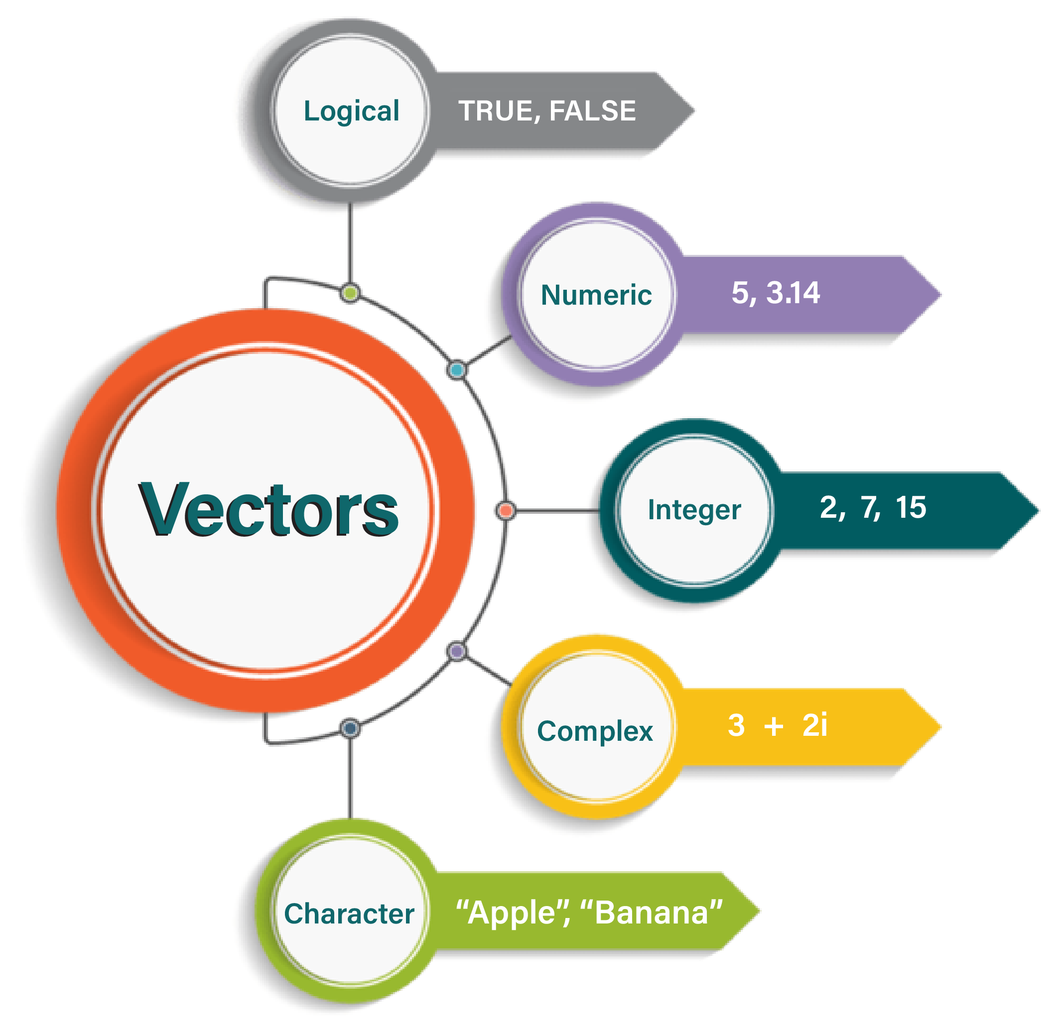
A vector is a one-dimensional array in R that stores elements of the same data type. Vectors are the most basic and frequently used data structures in R and are essential for data manipulation and analysis.
2.5.1 Creating a Vector
You can create a vector in R using the c() function1, which stands for “combine” or “concatenate.”
Example 1: Eye Colour
eye_colour <- c("Green", "Blue", "Brown", "Green", "Green", "Brown", "Blue")

eye_colour
#> [1] "Green" "Blue" "Brown" "Green" "Green" "Brown" "Blue"Here, eye_colour is a character vector, as it contains text values and the c() function makes it easy to combine individual elements into a single vector.
Best Practice:
When using the c() function, it’s a good practice to add a space after each comma. This makes your code cleaner and easier to read.
Example 2: Product Prices
# Vector of product prices in USD

product_prices <- c(19.99, 5.49, 12.89, 99.99, 49.95)

product_prices
#> [1] 19.99 5.49 12.89 99.99 49.952.5.2 Checking the Type of a Vector
To determine the data type of a vector, use the class() function:
class(product_prices)#> [1] "numeric"2.5.3 Length of a Vector
The length of a vector refers to the total number of elements it contains. You can determine this using the length() function, which returns an integer representing the total count of elements in the vector.
2.5.4 Advanced Vector Creation
While the simplest way to create a vector is by directly assigning values, R provides powerful tools for generating and manipulating vectors tailored to specific needs. This section explores advanced methods like :, c(), seq(), rep(), and sample() to create flexible, efficient, and custom vectors.
2.5.4.1 : Operator - Quick Sequence Generation
The : operator generates a sequence of integers between a starting and an ending value.
Syntax:
start:endWhere:
start: The starting value of the sequence.end: The ending value of the sequence.
Examples:
-
Create a sequence from 1 to 10:
sequence <- 1:10
sequence
#> [1] 1 2 3 4 5 6 7 8 9 10 -
Create a descending sequence:
reverse_sequence <- 10:1
reverse_sequence
#> [1] 10 9 8 7 6 5 4 3 2 1
Use Case
The : operator is ideal for quickly generating ranges for indexing, loops, or other operations requiring consecutive integers.
2.5.4.2 c() Function - Vector Concatenation
The c() function combines individual elements or existing vectors into a single vector.
Syntax:
c(element1, element2, ..., elementN)Where:
-
element1,element2, …,elementN: The individual values or vectors to be combined into a single vector.
Examples:
-
Combine numeric elements:
numbers <- c(2, 4, 6, 8)
numbers
#> [1] 2 4 6 8 -
Concatenate multiple vectors:
-
Combine mixed data types:
mixed <- c(10, "Apple", TRUE)
mixed
#> [1] "10" "Apple" "TRUE"
Use Case
All elements are coerced to the same data type (character in this case). Use c() to append data, merge multiple vectors, or build vectors from scratch.
2.5.4.3 seq() Function - Custom Sequence Generation
The seq() function allows for more flexible sequence generation compared to the : operator. You can specify the step size or desired length of the sequence.
Syntax:
seq(from, to, by, length)Where:
from: The starting value of the sequence.to: The ending value of the sequence.by: The increment (step size) between values. Defaults to1if not specified.length: The desired number of elements in the sequence. Overridesbyif specified.
Examples:
-
Generate a sequence with a positive step size:
custom_step <- seq(1, 10, by = 2)
custom_step
#> [1] 1 3 5 7 9 -
Generate a sequence with a negative non-integer step size:
descending <- seq(5, 1, by = -0.5)
descending
#> [1] 5.0 4.5 4.0 3.5 3.0 2.5 2.0 1.5 1.0 -
Generate a sequence of a specific length:
custom_length <- seq(1, 10, length = 5)
custom_length
#> [1] 1.00 3.25 5.50 7.75 10.00
Use Case
The seq() function is perfect for creating sequences with integer (non-integer) steps or evenly spaced data points.
2.5.4.4 rep() Function - Value Replication
The rep() function replicates values multiple times, creating patterns or duplications as needed.
Syntax:
rep(x, times, each)Where:
x: The vector or value to be replicated.times: The number of times to repeat the entire vector.each: The number of times to repeat each element of the vector.
Examples:
-
Repeat a value multiple times:
rep("God is good!", 5)#> [1] "God is good!" "God is good!" "God is good!" "God is good!" #> [5] "God is good!" -
Repeat a vector multiple times:
rep(1:3, times = 2)#> [1] 1 2 3 1 2 3 -
Repeat each element of a vector:
Use Case
Use rep() to generate repetitive patterns for simulation, modeling, or experimental data.
2.5.4.5 sample() Function - Random Sampling
The sample() function generates random samples from a vector, with or without replacement.
Syntax:
sample(x, size, replace = FALSE, prob = NULL)Where:
x: The vector to sample from.size: The number of samples to draw.replace: Logical; whether sampling is with replacement (TRUE) or without replacement (FALSE).prob: A vector of probabilities for each element inx.
Examples:
-
Random sample without replacement:
fruit <- c("Apple", "Banana", "Cherry", "Orange", "Pineapples", "Grape", "Pawpaw")

sample(x = fruit, size = 4)
#> [1] "Pawpaw" "Grape" "Apple" "Pineapples"Example output; results vary due to randomness
-
Random sample with replacement:
sample(1:10, 5, replace = TRUE)#> [1] 9 1 6 7 1Example output; results vary due to randomness
Set a Seed for Reproducibility
When you perform random sampling in R, the results may vary each time you run the code. By using set.seed(), you ensure that the random number generator starts from the same point, producing consistent results every time the code is executed.
Examples
# Set a seed for consistent results
set.seed(123)

# Generate a random sample of 5 numbers
sample(1:10, 5)
#> [1] 3 10 2 8 6This output will always be the same with set.seed(123)
-
Weighted Sampling:
Weighted sampling is a method of random sampling where each element in the population is assigned a probability of being selected. These probabilities, or weights, determine the likelihood of an element being chosen, allowing certain elements to have a higher or lower chance of selection compared to others.
Example:
Let’s simulate 10 flips of a biased coin, where the probability of getting a Head (H) is \(0.7\) and the probability of a Tail(T) is \(0.3\).
# Sample with probabilities

set.seed(1923)

coin_face <- c("H", "T") # Possible outcomes

prob <- c(0.7, 0.3) # Higher probability for "Head"

# Perform weighted sampling

sampled_prob <- sample(coin_face, prob = prob, size = 10, replace = TRUE)

sampled_prob
#> [1] "H" "H" "H" "H" "T" "T" "T" "T" "T" "H"
Use Case
Use sample() for bootstrapping, simulations, or creating random subsets from data.
2.5.5 Vector Operations
When working with vectors, most basic operations are applied element-by-element, making it both intuitive and efficient to transform and analyse collections of data.
2.5.5.1 Arithmetic Operations
Arithmetic operations on vectors are performed element-wise. For example, consider a vector of product prices:
# Vector of product prices in USD

product_prices <- c(19.99, 5.49, 12.89, 99.99, 49.95)
If we want to apply a \(10\%\) discount to all prices, we can multiply the entire vector by 0.9:
# Apply a discount of 10% to all product prices

discounted_prices <- product_prices * 0.9

discounted_prices
#> [1] 17.991 4.941 11.601 89.991 44.955In this example, each element in product_prices is multiplied by \(0.9\), producing the discounted_prices vector.
Common Pitfall
Data Type Coercion: Mixing data types in a vector can lead to unexpected results.
Tip: Ensure all elements are of the same data type to avoid automatic coercion.
2.5.5.2 Mathematical and Statistical Functions
R provides many built-in functions that operate on vectors and return summary values or transformed vectors. These functions are vectorised, meaning they automatically apply to every element where relevant. Examples include:
sum(product_prices)– returns the sum of all prices.mean(product_prices)– returns the average price.max(product_prices)/min(product_prices)– returns the maximum or minimum value.sd(product_prices)/var(product_prices)– returns the standard deviation or variance of the product prices.round(product_prices, digits = 1)– rounds all prices to one decimal place.
2.5.5.3 Element-wise Functions
Functions like sqrt(), log(), exp(), and abs() apply mathematically to each element:
2.5.5.4 Sorting and Ordering
You can also sort vectors or determine the order of elements:
2.5.5.5 Vectorised Conditional Operations with ifelse()
The ifelse() statement is a vectorised conditional function in R. It evaluates a condition for each element of a vector, returning one value if the condition is TRUE and another value if it is FALSE. This makes it an essential function for data transformation and analysis.
Example 1: Categorise Product Prices
Suppose we have a vector of product prices in USD, and we want to categorise them as “Affordable” or “Expensive” based on whether they are below or above $50.
# Vector of product prices in USD
product_prices <- c(30, 75, 50, 20, 100)

# Categorise prices as "Affordable" or "Expensive"
price_category <- ifelse(product_prices < 50, "Affordable", "Expensive")

# Print the result
price_category
#> [1] "Affordable" "Expensive" "Expensive" "Affordable" "Expensive"Example 2: Apply a Discount for Expensive Products
If a product price is above $50, apply a 10% discount. Otherwise, keep the price unchanged.
# Apply discount for products above $50
discounted_prices <- ifelse(product_prices > 50, product_prices * 0.9, product_prices)

# Print the result
discounted_prices
#> [1] 30.0 67.5 50.0 20.0 90.02.5.6 Vector selection
To select elements of a vector, use square brackets [] with the index of the element(s). R indexing starts at 1 (i.e. R uses 1-based indexing).
For example:
| Weekday | Monday | Tuesday | Wednesday | Thursday | Friday | Saturday | Sunday |
|---|---|---|---|---|---|---|---|
| index | 1 | 2 | 3 | 4 | 5 | 6 | 7 |
Example 1
weekday <- c(
  "Monday", "Tuesday", "Wednessday", "Thursday", "Friday", "Saturday", "Sunday"
)
Access the first weekday:
weekday[1]#> [1] "Monday"Access the second weekday:
weekday[2]#> [1] "Tuesday"Access multiple elements
weekday[c(2, 4)]#> [1] "Tuesday" "Thursday"2.5.7 Reflection Question 2.1.1
Why is it important to know that R uses 1-based indexing?
See the Solution to Reflection Question 2.1.1
In addition to selecting elements by their positions, you can select elements of a vector based on conditions using comparison operators. This method involves creating a logical vector of TRUE and FALSE values by applying a condition to the vector, and then using this logical vector to index the original vector.
Example 2
Let’s start with a numeric vector representing daily temperatures:
# Create a numeric vector of temperatures
temperatures <- c(72, 65, 70, 68, 75, 80, 78)
Select temperatures greater than 70 degrees:
# Apply the condition and select elements
temperatures[temperatures > 70]
#> [1] 72 75 80 78
Explanation
temperatures > 70creates a logical vector:[TRUE, FALSE, FALSE, FALSE, TRUE, TRUE, TRUE].temperatures[temperatures > 70]selects elements where the condition isTRUE.
Select temperature that are even.
temperatures[temperatures %% 2 == 0]#> [1] 72 70 68 80 78
Explanation
temperatures %% 2computes the remainder when each temperature is divided by 2.temperatures %% 2 == 0returnsTRUEfor even temperature.
Example 3
Using our weekday vector:
weekday <- c(
  "Monday", "Tuesday", "Wednesday", "Thursday", "Friday",
  "Saturday", "Sunday"
)
Select weekdays that are “Saturday” or “Sunday”:
# Create a logical vector for the condition
is_weekend <- weekday == "Saturday" | weekday == "Sunday"

# Select elements based on the condition
weekend_days <- weekday[is_weekend]

# Display the result
weekend_days
#> [1] "Saturday" "Sunday"
Explanation
weekday == "Sunday"returns[FALSE, FALSE, FALSE, FALSE, FALSE, FALSE, TRUE].Using
|(logical OR) combines the two conditions.The final logical vector is
[FALSE, FALSE, FALSE, FALSE, FALSE, TRUE, TRUE].
Selecting Weekdays (Excluding Weekends)
# Create a logical vector for weekdays
is_weekday <- !(weekday %in% c("Saturday", "Sunday"))

# Select elements based on the condition
weekday_days <- weekday[is_weekday]

# Display the result
weekday_days
#> [1] "Monday" "Tuesday" "Wednesday" "Thursday" "Friday"
Explanation
weekday %in% c("Saturday", "Sunday")checks if each element is in the vectorc("Saturday", "Sunday").The
%in%operator returns[FALSE, FALSE, FALSE, FALSE, FALSE, TRUE, TRUE].Using
!negates the logical vector to[TRUE, TRUE, TRUE, TRUE, TRUE, FALSE, FALSE].
Code Style Guidelines
Naming Conventions: Use descriptive variable names in
snake_case.Indentation: Use consistent indentation for readability.
Comments: Explain complex code with comments.
2.5.8 Exercise 2.1.1: Vector Selection
Given the monthly sales figures (in units) for a product over a year:
120, 135, 150, 160, 155, 145, 170, 180, 165, 175, 190, 200
Your Tasks:
Create a vector named
monthly_salescontaining the data.Access the sales figures for March, June, and December.
Find the sales figures that are less than 60
Calculate the average sales for the first quarter (January to March).
Extract the sales figures for the last month of each quarter of the year
2.5.9 Factor Vectors
Factors are a fundamental data structure in R used to represent categorical variables, where each value belongs to a specific category or “level.” Unlike character vectors, factors store categorical data more efficiently and are essential in statistical modeling, especially when using functions like summary() or performing analyses that require categorical distinctions.
2.5.9.1 Why Use Factors?
Statistical Modeling: Factors are crucial in statistical modeling as they explicitly designate categorical variables, allowing R’s modeling functions to handle them appropriately.
Efficient Storage: Factors store categorical data more efficiently than character vectors by using integer codes under the hood.
Data Integrity: By restricting data to predefined categories (levels), factors help maintain data integrity and reduce errors due to invalid entries.
Using Factors in Plots: Factors are particularly useful when creating plots, as they allow for meaningful ordering of categories.
2.5.9.2 Creating a Factor Vector
You can create a factor vector using the factor() function, converting a character or numeric vector into a factor.
Example 1: Product Categories
Suppose we have a vector of product categories:
# Vector of product categories
product_categories <- c(
  "Electronics", "Clothing", "Electronics",
  "Furniture", "Clothing", "Electronics"
)

product_categories
#> [1] "Electronics" "Clothing" "Electronics" "Furniture" "Clothing"
#> [6] "Electronics"Converting to a factor:
# Convert to factor
product_categories_factor <- factor(product_categories)

# Display the factor vector
product_categories_factor
#> [1] Electronics Clothing Electronics Furniture Clothing Electronics
#> Levels: Clothing Electronics FurnitureInspecting the Factor Levels:
levels(product_categories_factor)#> [1] "Clothing" "Electronics" "Furniture"Checking the Data Type:
class(product_categories_factor)#> [1] "factor"If you already have a character vector, you can convert it to a factor vector using the as.factor() function.
Example 2: Ethnicity Categories
ethnicity <- c(
  "African", "Asian", "Latin American", "African", "Latin American",
  "Asian", "African", "European"
)

ethnicity_factor <- as.factor(ethnicity)

ethnicity_factor
#> [1] African Asian Latin American African
#> [5] Latin American Asian African European
#> Levels: African Asian European Latin American
Note
The levels are automatically determined and sorted alphabetically unless specified otherwise.
2.5.9.3 Ordered Factors
Sometimes, categorical variables have a natural ordering (e.g., “Low” < “Medium” < “High”). In such cases, you can create an ordered factor by specifying the levels in the desired order and setting ordered = TRUE.
Example 3: Satisfaction Ratings
# Vector of satisfaction ratings

satisfaction_ratings <- c(
  "High", "Medium", "Low", "High",
  "Medium", "Low", "High"
)

# Create an ordered factor
satisfaction_factors <- factor(satisfaction_ratings,
  levels = c("Low", "Medium", "High"),
  ordered = TRUE
)

# Display the ordered factor
satisfaction_factors
#> [1] High Medium Low High Medium Low High
#> Levels: Low < Medium < HighChecking the data type:
class(satisfaction_factors)#> [1] "ordered" "factor"
2.5.9.4 Using summary() with Factors:
The summary() function provides a count of each category in a factor vector:
# Summarise the satisfaction factors

summary(satisfaction_factors)
#> Low Medium High
#> 2 2 32.5.9.5 Converting Factors to Numeric Values
Be cautious when converting factors to numeric values. Direct conversion using as.numeric() will return the internal integer codes representing the factor levels, which may not correspond to the actual values you expect.
Incorrect Way:
# Incorrect conversion
as.numeric(product_categories_factor)
#> [1] 2 1 2 3 1 2
Tip
The numbers represent the position of each level in the levels attribute, not the original data.
Correct Way:
First, convert the factor to a character vector, then to numeric (if applicable):
# Correct conversion (if levels are numeric strings)
as.numeric(as.character(product_categories_factor))
#> Warning: NAs introduced by coercion#> [1] NA NA NA NA NA NA
Warning
This will produce NAs because the levels are not numeric strings. For factors with numeric levels, this method works correctly.
Example with Numeric Levels:
# Numeric factor example
numeric_factor <- factor(c("1", "3", "5", "2"))

# Correct conversion
numeric_values <- as.numeric(as.character(numeric_factor))

numeric_values
#> [1] 1 3 5 2
Common Pitfalls
-
Unintended Ordering: By default, factors are unordered. If your categorical variable has a natural order, specify it using the
levelsargument and setordered = TRUE. Converting Factors: Always be cautious when converting factors to numeric types to avoid unexpected results. Use
as.character()beforeas.numeric()if necessary.-
Missing Levels: If you specify levels that are not present in your data, R will include them with a count of zero.
feedback_ratings <- c(
  "Good", "Excellent", "Poor", "Fair",
  "Good", "Excellent", "Fair"
)

# Specifying extra levels
feedback_factors <- factor(feedback_ratings,
  levels = c("Poor", "Fair", "Good", "Very Good", "Excellent"),
  ordered = TRUE
)

# Summarise
summary(feedback_factors)
#> Poor Fair Good Very Good Excellent #> 1 2 2 0 2
Ensure that the levels you specify match the data or be aware that additional levels will appear with zero counts.
2.5.9.6 Removing Unused Factor Levels
When working with factors in R, you might encounter situations where, after subsetting your data, the factor levels still include categories that no longer exist in your dataset. These unused levels can lead to misleading analyses and cluttered visualizations. To ensure that your factor variables accurately reflect the data, it’s important to remove these unused levels. This can be easily achieved using the droplevels() function.
Why Remove Unused Levels?
Accurate Analysis: Statistical functions and models may misinterpret unused levels, affecting results.
Clean Visualizations: Plots and charts can display empty categories, making them confusing.
Data Integrity: Keeping only relevant levels ensures your data accurately represents the current state.
Example 1: Removing Unused Levels from a Factor
Suppose you have a factor vector representing customer feedback ratings:
# Original factor with all levels
feedback_ratings <- c(
  "Good", "Excellent", "Poor",
  "Fair", "Good", "Excellent", "Fair"
)

feedback_factors <- factor(feedback_ratings,
  levels = c("Poor", "Fair", "Good", "Excellent"),
  ordered = TRUE
)

# Display the original factor
feedback_factors
#> [1] Good Excellent Poor Fair Good Excellent Fair
#> Levels: Poor < Fair < Good < ExcellentNow, you decide to exclude the “Poor” ratings from your analysis:
# Subset the data to exclude "Poor" ratings
subset_feedback <- feedback_factors[feedback_factors != "Poor"]

# Display the subsetted factor
subset_feedback
#> [1] Good Excellent Fair Good Excellent Fair
#> Levels: Poor < Fair < Good < Excellent
Observation
Even after subsetting, the level “Poor” remains in the levels attribute, despite not being present in the data.
Using droplevels() to Remove Unused Levels
To clean up the factor and remove any levels that are no longer used, apply the droplevels() function:
# Remove unused levels
subset_feedback <- droplevels(subset_feedback)

# Display the cleaned factor
subset_feedback
#> [1] Good Excellent Fair Good Excellent Fair
#> Levels: Fair < Good < ExcellentNow, the factor levels accurately reflect only the categories present in the data.
# Check the levels of the cleaned factor
levels(subset_feedback)
#> [1] "Fair" "Good" "Excellent"
Note
Always Check Levels After Subsetting: It’s good practice to check the levels of your factor variables after any subsetting operation.
# Check levels before and after dropping unused levels
levels(feedback_factors)
#> [1] "Poor" "Fair" "Good" "Excellent"levels(subset_feedback)#> [1] "Fair" "Good" "Excellent"Apply droplevels() to Data Frames: If your data frame contains factor columns and you’ve performed row-wise subsetting, you can apply droplevels() to the entire data frame to clean all factor columns at once.
# Assuming 'df' is your data frame
df_clean <- droplevels(df)
Use in Modeling and Visualization: Clean factor levels ensure that statistical models and plots accurately represent your data without misleading categories.
2.5.10 Reflection Question 2.1.2
How does converting character vectors to factors benefit data analysis in R?
When would you use a factor instead of a character vector in R?
2.5.11 Practice Quiz 2.1
Question 1:
Which function is used to create a vector in R?
Question 2:
Given the vector:
v <- c(2, 4, 6, 8, 10)
What is the result of v * 3?
-
c(6, 12, 18, 24, 30)
-
c(2, 4, 6, 8, 10, 3)
-
c(6, 12, 18, 24)
- An error occurs
Question 3:
In R, is the vector c(TRUE, FALSE, TRUE) considered a numeric vector?
- True
- False
Question 4:
What will be the output of the following code?
numbers <- c(1, 3, 5, 7, 9)
numbers[2:4]-
1, 3, 5
-
3, 5, 7
-
5, 7, 9
2, 4, 6
Question 5:
Which of the following best describes a factor in R?
- A numerical vector
- A categorical variable with predefined levels
- A two-dimensional data structure
- A list of vectors
Question 6:
Which function is used to create sequences including those with either integer or non-integer steps?
Question 7:
What does the following code output?
seq(10, 1, by = -3)-
10, 7, 4, 1
-
10, 7, 4
-
1, 4, 7, 10
- An error occurs
Question 8:
Suppose you want to create a vector that repeats the sequence 1, 2, 3 five times. Which code will achieve this?
-
rep(c(1, 2, 3), each = 5)
-
rep(c(1, 2, 3), times = 5)
-
rep(1:3, times = 5)
rep(1:3, each = 5)
Question 9:
Suppose you are drawing coins from a treasure chest. There are 100 coins in this chest: 20 gold, 30 silver, and 50 bronze. Use R to draw 5 random coins from the chest. Use set.seed(50) to ensure reproducibility.
What will be the output of the random draw?
Silver, Bronze, Bronze, Bronze, Silver-
Gold, Gold, Silver, Bronze, Bronze
-
Gold, Bronze, Bronze, Bronze, Silver
Silver, Bronze, Gold, Bronze, Bronze
Question 10:
What will the following code produce?
-
5, 7, 8
-
5, 7, 7
- An error due to unequal vector lengths
5, 7, 9
2.5.12 Exercise 2.1.2: Vector and Factor Manipulation
Given a vector of customer feedback ratings: c("Good", "Excellent", "Poor", "Fair", "Good", "Excellent", "Fair")
Your Tasks:
Create a vector named
feedback_ratingscontaining the data.Convert
feedback_ratingsinto an ordered factor with levels: “Poor” < “Fair” < “Good” < “Excellent”.Summarize the feedback ratings.
Identify how many customers rated “Excellent”.
2.6 Experiment 2.2: Matrices
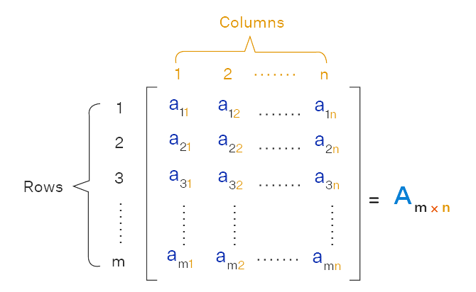
A matrix is a two-dimensional data structure consisting of a rectangular array of elements of the same data type, organized into rows and columns. Matrices are used extensively in linear algebra and statistical computations. Figure 2.3 illustrates a typical representation of a matrix.
2.6.1 Creating Matrices
To create a matrix, use the matrix() function:
#|
matrix(data, nrow, ncol, byrow = FALSE)
where:
data: The elements to be arranged in the matrix.nrow: The number of rows.ncol: The number of columns.byrow: If set toFALSE(the default), fills the matrix by columns; if set toTRUE, fills the matrix by rows.
Create the matrix A:
\[A = \begin{pmatrix} 1&-2& 5\\ -3&9&4\\ 5&0&6 \end{pmatrix}\]
#>      [,1] [,2] [,3]
#> [1,]    1   -2    5
#> [2,]   -3    9    4
#> [3,]    5    0    6
Create the matrix B:
\[B = \begin{pmatrix} 2&-8& 14\\ 4&10&16\\ 6&12&18 \end{pmatrix}\]
2.6.2 Matrices slicing
Accessing elements in a matrix is done by using [row, column], between the square brackets, you indicate the position of the row and column in which the elements to access are. For example, to access the element in the first row and second column of matrix A, you type A[1, 2]. To access the element in the third row and second column of matrix A, you type A[3, 2].
A[1, 2] # Element in first row, second column#> [1] -2A[3, 2] # Element in third row, second column#> [1] 02.6.3 Arithmetic Operation in Matrices
You can perform arithmetic operations on matrices. Consider the following matrices
\[A = \begin{pmatrix} 1&-2& 5\\ -3&9&4\\ 5&0&6 \end{pmatrix}\]
\[B = \begin{pmatrix} 2&-8& 14\\ 4&10&16\\ 6&12&18 \end{pmatrix}\]
Addition
A + B#> [,1] [,2] [,3]
#> [1,] 3 6 19
#> [2,] 1 19 20
#> [3,] 11 12 24Multiplication
Matrix multiplication is done using %*% operator:
A %*% B#> [,1] [,2] [,3]
#> [1,] 24 48 72
#> [2,] 54 114 174
#> [3,] 46 112 1782.6.4 Exercise 2.2.1: Matrix Transpose
Consider the following matrix \(A\):
\[A = \begin{pmatrix} 1 & 3 & 5 \\ 2 & 4 & 6 \end{pmatrix}\]
Your Task:
Find the transpose of matrix \(A\), denoted as \(A^{T}\).
Tip
Define matrix \(A\), then use t(A) to find its transpose.
Here’s a starting point for your code:
Replace the ... with the correct values and complete the exercise!
2.6.5 Exercise 2.2.2: Matrix Inverse Multiplication
Given the matrices \(A\) and \(B\) below:
\[A = \begin{pmatrix} 4 & 7 \\ 2 & 6 \end{pmatrix}\]
\[ B = \begin{pmatrix} 3 & 5 \\ 1 & 2 \end{pmatrix}\]
Your Task:
Calculate \(A^{-1} \times B\), where \(A^{-1}\) is the inverse of matrix \(A\).
Hint:
Use the
solve()function in R to find the inverse of matrix \(A\).Use the matrix multiplication operator
%*%to multiply \(A^{-1}\) by \(B\).
Here’s a starting point for your code:
Replace the ... with the correct values for your matrices and complete the exercise!
2.6.6 Real-World Data Scenario: Sales Data Matrix
Suppose we have sales data for three products over four regions.
# Sales data (units sold)

sales_data <- c(500, 600, 550, 450, 620, 580, 610, 490, 530, 610, 570, 480)

# Create a matrix

sales_matrix <- matrix(sales_data, nrow = 4, ncol = 3, byrow = TRUE)

colnames(sales_matrix) <- c("Product_A", "Product_B", "Product_C")

rownames(sales_matrix) <- c("Region_1", "Region_2", "Region_3", "Region_4")

sales_matrix
#> Product_A Product_B Product_C
#> Region_1 500 600 550
#> Region_2 450 620 580
#> Region_3 610 490 530
#> Region_4 610 570 480Addition and Subtraction:
# Assume a competitor's sales matrix
competitor_sales <- matrix(
  c(
    480, 590, 540, 430, 610, 570,
    600, 480, 520, 600, 560, 470
  ),
  nrow = 4, ncol = 3, byrow = TRUE
)

competitor_sales
#> [,1] [,2] [,3]
#> [1,] 480 590 540
#> [2,] 430 610 570
#> [3,] 600 480 520
#> [4,] 600 560 470# Calculate the difference in sales
sales_difference <- sales_matrix - competitor_sales
sales_difference#> Product_A Product_B Product_C
#> Region_1 20 10 10
#> Region_2 20 10 10
#> Region_3 10 10 10
#> Region_4 10 10 10Matrix Multiplication:
# Price per product
prices <- c(20, 15, 25)

# Calculate total revenue per region

revenue_per_region <- sales_matrix %*% prices
revenue_per_region
#> [,1]
#> Region_1 32750
#> Region_2 32800
#> Region_3 32800
#> Region_4 32750Accessing Elements:
# Sales of Product_B in Region_2
sales_matrix["Region_2", "Product_B"] # Returns 580
#> [1] 620# All sales for Product_C
sales_matrix[, "Product_C"]#> Region_1 Region_2 Region_3 Region_4
#> 550 580 530 480
Common Pitfall
-
Dimension Mismatch:
- Tip: Ensure that the number of columns in the first matrix matches the number of rows in the second for multiplication.
2.6.7 Reflection Question 2.2.1
- In what scenarios would using a matrix be more advantageous than a data frame?
2.6.8 Practice Quiz 2.2
Question 1:
Which R function is used to find the transpose of a matrix?
-
transpose()
-
t()
-
flip()
reverse()
Question 2:
Given the matrix:
A <- matrix(1:6, nrow = 2, byrow = TRUE)
what is the value of A[2, 3]?
- 3
- 6
- 5
- 4
Question 3:
Matrix multiplication in R can be performed using the * operator.
True
False
Question 4:
What will be the result of adding two matrices of different dimensions in R?
- R will perform element-wise addition up to the length of the shorter matrix.
- An error will occur due to dimension mismatch.
- R will recycle elements of the smaller matrix.
- The matrices will be concatenated.
Question 5:
Which function can be used to calculate the sum of each column in a matrix M?
-
rowSums(M)
-
colSums(M)
-
sum(M)
apply(M, 2, sum)
Question 6:
Which function is used to create a matrix in R?
2.6.9 Exercise 2.2.3: Matrix Operations
Using the sales_matrix from the example in Section 2.6.6:
- Calculate the total units sold per product.
- Find the average units sold across all regions for
Product_A. - Identify the region with the highest sales for
Product_C.
2.7 Experiment 2.3: Data frame
A data frame is a two-dimensional data structure. It resembles a table, where variables are represented as columns, and observations are rows—much like a spreadsheet or a SQL table. Data frames allow you to store columns of different data types (e.g., numeric, character, logical), making them ideal for real-world datasets.
2.7.1 Creating a Data Frame
To create a data frame, use the data.frame() function.
Example 1: Sales Transactions Data Frame
# Sample sales transactions
transaction_id <- 1:5

product <- c("Product_A", "Product_B", "Product_C", "Product_A", "Product_B")

quantity <- c(2, 5, 1, 3, 4)

price <- c(19.99, 5.49, 12.89, 19.99, 5.49)

total_amount <- quantity * price

sales_transactions <- data.frame(
  transaction_id, product, quantity, price,
  total_amount
)

sales_transactions
#> transaction_id product quantity price total_amount
#> 1 1 Product_A 2 19.99 39.98
#> 2 2 Product_B 5 5.49 27.45
#> 3 3 Product_C 1 12.89 12.89
#> 4 4 Product_A 3 19.99 59.97
#> 5 5 Product_B 4 5.49 21.96Notice the row numbers (1 2 3 4 5) displayed on the left of the console output—these are row labels. Each column in a data frame is internally represented as a vector.
Example 2: COVID 19 Data Frame
You can create a data frame for COVID-19 statistics with columns such as states, confirmed_cases, recovered_cases, and death_cases:
states <- c("Lagos", "FCT", "Plateau", "Kaduna", "Rivers", "Oyo")
confirmed_cases <- c(58033, 19753, 9030, 8998, 7018, 6838)
recovered_cases <- c(56990, 19084, 8967, 8905, 6875, 6506)
death_cases <- c(439, 165, 57, 65, 101, 123)
covid_19 <- data.frame(states, confirmed_cases, recovered_cases, death_cases)
covid_19#> states confirmed_cases recovered_cases death_cases
#> 1 Lagos 58033 56990 439
#> 2 FCT 19753 19084 165
#> 3 Plateau 9030 8967 57
#> 4 Kaduna 8998 8905 65
#> 5 Rivers 7018 6875 101
#> 6 Oyo 6838 6506 1232.7.2 Exploring Data Frames
R provides several functions to quickly explore the structure and content of data frame (df):
head(df): Displays the first few rows.tail(df): Displays the last few rows.
Both functions also include a “header”, showing the variable names in the data frame`.
-
str(df): Shows the structure of the data frame, including:Number of observations (rows) and variables (columns).
Variable names and data types.
A preview of the data in each column.
names(df): Lists the names of the columns.nrow(df): Returns the number of rows.ncol(df): Returns the number of columns.dim(df): Returns the dimensions (rows and columns) as a vector.View(df): Opens a spreadsheet-style viewer in RStudio.summary(df): Provides summary statistics for all columns.
Example: Medical Data Frame
Consider the following vectors:
Exploring the Medical Data Frame
First six observations:
head(medical_data)#> gender height weight bmi
#> 1 Male 3 47 5.222222
#> 2 Female 2 46 11.500000
#> 3 Female 3 58 6.444444
#> 4 Female 2 64 16.000000
#> 5 Male 3 62 6.888889
#> 6 Female 2 53 13.250000Last six observations:
tail(medical_data) # To get the last 6 observation#> gender height weight bmi
#> 115 Male 2 54 13.500000
#> 116 Male 3 66 7.333333
#> 117 Male 3 57 6.333333
#> 118 Male 3 49 5.444444
#> 119 Male 2 51 12.750000
#> 120 Female 3 51 5.666667Column names:
names(medical_data)#> [1] "gender" "height" "weight" "bmi"You can also use:
colnames(medical_data)#> [1] "gender" "height" "weight" "bmi"View the data in RStudio (interactive):
View(medical_data)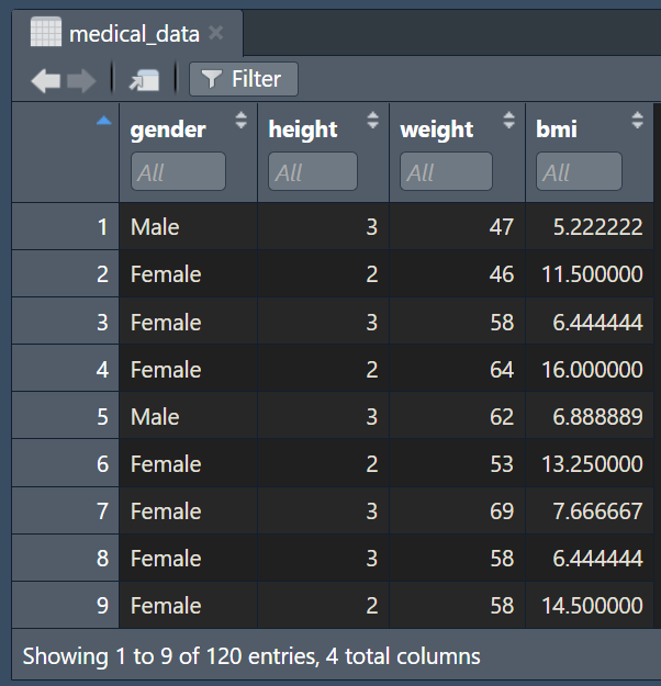
Descriptive statistics:
summary(medical_data)#> gender height weight bmi
#> Length:120 Min. :1.000 Min. :37.00 Min. : 2.375
#> Class :character 1st Qu.:2.000 1st Qu.:50.00 1st Qu.: 6.333
#> Mode :character Median :2.000 Median :56.00 Median :11.000
#> Mean :2.433 Mean :55.58 Mean :12.384
#> 3rd Qu.:3.000 3rd Qu.:62.00 3rd Qu.:14.312
#> Max. :4.000 Max. :78.00 Max. :63.0002.7.3 Built-in Datasets
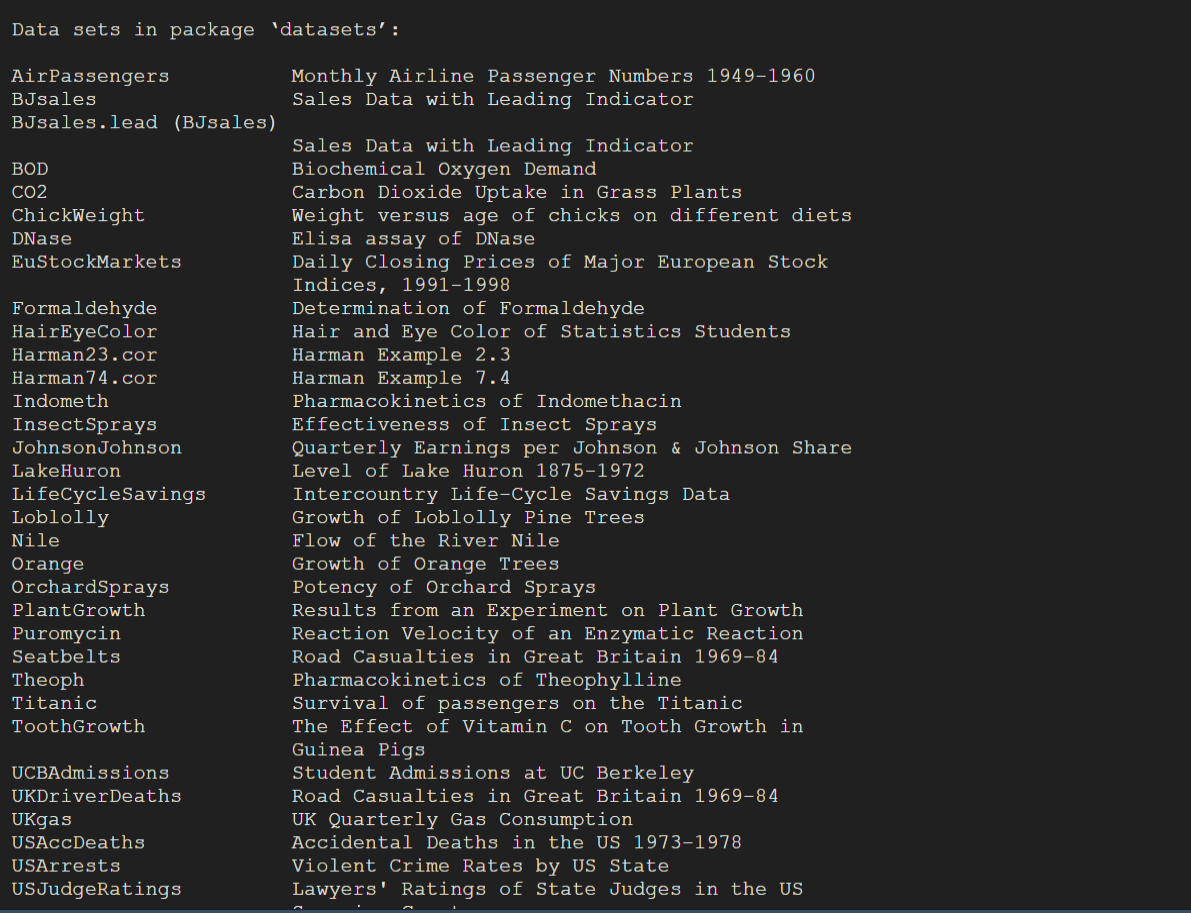
R comes with a variety of built-in datasets that you can use for learning, testing, or exploring data analysis techniques. To view the available datasets, use the following command:
data()This will open a list of all the datasets available in the datasets package. The datasets package provides a variety of datasets on different topics, such as biology, finance, and historical events. Figure 2.5 is an example output showing some of these datasets:
2.7.3.1 Loading and Previewing Datasets
You can load and preview built-in datasets simply by calling their names. For example:
head(iris)#> Sepal.Length Sepal.Width Petal.Length Petal.Width Species
#> 1 5.1 3.5 1.4 0.2 setosa
#> 2 4.9 3.0 1.4 0.2 setosa
#> 3 4.7 3.2 1.3 0.2 setosa
#> 4 4.6 3.1 1.5 0.2 setosa
#> 5 5.0 3.6 1.4 0.2 setosa
#> 6 5.4 3.9 1.7 0.4 setosaThis displays the first six rows of the iris dataset, which contains measurements of iris flowers.
head(airquality)#> Ozone Solar.R Wind Temp Month Day
#> 1 41 190 7.4 67 5 1
#> 2 36 118 8.0 72 5 2
#> 3 12 149 12.6 74 5 3
#> 4 18 313 11.5 62 5 4
#> 5 NA NA 14.3 56 5 5
#> 6 28 NA 14.9 66 5 6Here, the airquality dataset provides daily air quality measurements in New York from May to September 1973.
2.7.3.2 Getting Help on a Dataset
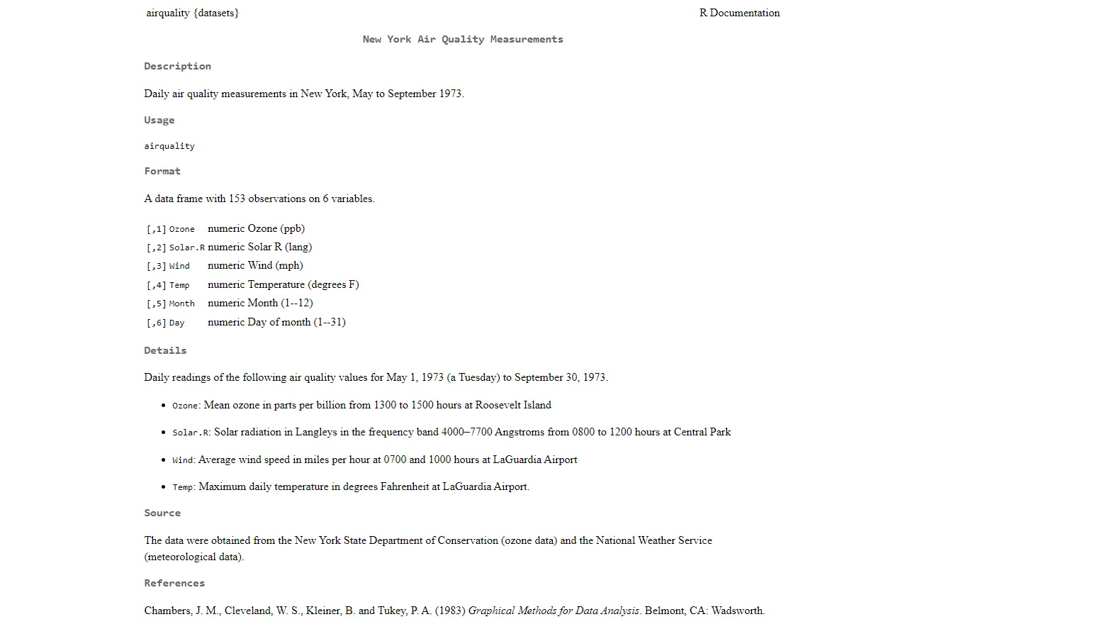
To learn more about a specific dataset, use the ? operator followed by the dataset name. For example:
?airqualityThis will bring up the documentation for the airquality dataset as shown in Figure 2.6, which includes details about the variables, their format, and the source of the data.
2.7.4 Subsetting Data Frames
Every column in a data frame has a name. You can view the column names of a data frame, such as iris, by using the names() function:
names(iris)#> [1] "Sepal.Length" "Sepal.Width" "Petal.Length" "Petal.Width"
#> [5] "Species"
2.7.4.1 Using the $ Operator
To access a specific column by name, use the $ operator in the format df$colname, where df is the name of the data frame and colname is the name of the column you want to retrieve. This operation returns the column as a vector. For example, to extract the Sepal.Length column from the iris data frame as a vector:
iris$Sepal.Length#> [1] 5.0 6.0 5.0 5.7 4.9 6.7 6.3 4.8 7.7 5.8 7.3 5.2 6.3 5.0 5.1 5.6 7.7 6.9
#> [19] 6.1 7.6Similarly, to access the Species column:
iris$Species#> [1] setosa versicolor virginica setosa virginica setosa
#> [7] versicolor setosa versicolor setosa virginica versicolor
#> [13] setosa virginica setosa versicolor virginica setosa
#> [19] setosa versicolor
#> Levels: setosa versicolor virginica
Note
For clarity and conciseness, we have shortened the output of both iris$Sepal.Length and iris$Species in the example outputs to save space. Both methods extract their respective columns as vectors.
Since the $ operator produces a vector, you can directly apply vector-based functions, such as mean(), sd(), or table(), to perform calculations on the column data.
For example:
- To compute the mean of
Sepal.Length:
mean(iris$Sepal.Length)#> [1] 5.843333- To find the frequency of each
Species:
table(iris$Species)#>
#> setosa versicolor virginica
#> 50 50 50
2.7.4.2 Using [row, column] Notation
You can also subset data frames using [row, column], similar to matrices. In this syntax:
The
rowargument specifies which rows to extract.The
columnargument specifies which columns to extract.
Here are some common examples and their interpretations, summarized in Table 2.1 below:
| Data Frame Slicing | Interpretation |
|---|---|
data[1, ] |
First row and all columns |
data[, 2] |
All rows and second column |
data[c(1, 3, 5), 2] |
Rows 1, 3, 5 and column 2 only |
data[1:3, c(1, 3)] |
First three rows and columns 1 and 3 only |
data or data[, ]
|
All rows and all columns |
Reflection Question 2.3.1
How does subsetting data frames help in data analysis?
Common Pitfalls
-
Undefined Columns Selected:
-
Tip: Use
names(df)to verify column names before subsetting.
-
Tip: Use
-
Incorrect Data Types:
-
Tip: Check data types with
str(df)and convert if necessary.
-
Tip: Check data types with
2.7.5 Practice Quiz 2.3
Question 1:
Which function would you use to view the structure of a data frame, including its data types and a preview of its contents?
Question 2:
How do you access the third row and second column of a data frame df?
-
df[3, 2]
-
df[[3, 2]]
-
df$3$2
df(3, 2)
Question 3:
In a data frame, all columns must contain the same type of data.
True
False
Question 4:
Which of the following commands would open a spreadsheet-style viewer of the data frame df in RStudio?
-
View(df)
-
view(df)
-
inspect(df)
display(df)
Question 5:
What does the summary() function provide when applied to a data frame?
- Only the first few rows of the data frame.
- Descriptive statistics for each column.
- The structure of the data frame including data types.
- A visual plot of the data.
Question 6:
In a data frame, all columns must be of the same data type.
True
False
2.7.6 Exercise 2.3.1: Subsetting a Dataframe
Using the built-in airquality dataset, complete the following tasks:
Examine the
airqualitydataset.Select the first three columns.
Select rows 1 through 3 and columns 1 and 3.
Select rows 1 through 5 and column 1.
Select the first row.
Select the first six rows.
2.7.7 Exercise 2.3.2: Data Frame Manipulation
Using the sales_transactions data frame:
# Sample sales transactions
transaction_id <- 1:5
product <- c("Product_A", "Product_B", "Product_C", "Product_A", "Product_B")
quantity <- c(2, 5, 1, 3, 4)
price <- c(19.99, 5.49, 12.89, 19.99, 5.49)
total_amount <- quantity * price
sales_transactions <- data.frame(
transaction_id, product, quantity,
price, total_amount
)
sales_transactions#> transaction_id product quantity price total_amount
#> 1 1 Product_A 2 19.99 39.98
#> 2 2 Product_B 5 5.49 27.45
#> 3 3 Product_C 1 12.89 12.89
#> 4 4 Product_A 3 19.99 59.97
#> 5 5 Product_B 4 5.49 21.96Add a new column
discounted_pricethat applies a 10% discount toprice.Filter transactions where the
total_amountis greater than $50.Calculate the average
total_amountforProduct_B.
2.8 Experiment 2.4: Lists
A list is an R object that can contain elements of different types—numbers, strings, vectors, and even other lists. It’s basically a container that can hold many different kinds of data structures.
You are already familiar with the notion of dimensions, such as the rows and columns in matrices and data frames. Unlike matrices or data frames, lists do not have the same concept of rows and columns. Instead, they are regarded as one-dimensional because they essentially consist of a sequence of items. You can think of it like a box full of different objects, all lined up one after the other.
2.8.1 Creating a List
To create a list, use the list() function:
# Customer Profile
customer_profile <- list(
customer_id = 1001,
name = "Johnny Drille",
purchase_history = sales_transactions, # A data frame in Exercise 2.3.2
loyalty_member = TRUE
)
customer_profile#> $customer_id
#> [1] 1001
#>
#> $name
#> [1] "Johnny Drille"
#>
#> $purchase_history
#>   transaction_id   product quantity price total_amount
#> 1              1 Product_A        2 19.99        39.98
#> 2              2 Product_B        5  5.49        27.45
#> 3              3 Product_C        1 12.89        12.89
#> 4              4 Product_A        3 19.99        59.97
#> 5              5 Product_B        4  5.49        21.96
#>
#> $loyalty_member
#> [1] TRUEHere, customer_profile consists of four components:
customer_id: Numeric value.name: Character string.purchase_history: Data frameloyalty_member: Logical value.
To check how many elements are in a list, you can use the length() function. For instance:
length(customer_profile)#> [1] 42.8.2 Accessing List Elements
To show the contents of a list you can simply type its name as any other object in R:
customer_profile#> $customer_id
#> [1] 1001
#>
#> $name
#> [1] "Johnny Drille"
#>
#> $purchase_history
#>   transaction_id   product quantity price total_amount
#> 1              1 Product_A        2 19.99        39.98
#> 2              2 Product_B        5  5.49        27.45
#> 3              3 Product_C        1 12.89        12.89
#> 4              4 Product_A        3 19.99        59.97
#> 5              5 Product_B        4  5.49        21.96
#>
#> $loyalty_member
#> [1] TRUE-
Using
$Operator:
The$operator is used to access elements of a list by their names. This method is straightforward and commonly used when you know the exact name of the element you want to access.customer_profile$name#> [1] "Johnny Drille" -
Using Double Square Brackets
[[ ]]:
Double square brackets[[ ]]are used to extract elements from a list by their position (index) or name.customer_profile[[1]]#> [1] 1001customer_profile[["customer_id"]]#> [1] 1001 -
Using single square brackets
[]:
Using single square brackets [ ] returns a list containing the element:customer_profile[1]#> $customer_id #> [1] 1001customer_profile["customer_id"]#> $customer_id #> [1] 1001 -
Accessing Data Frame within List:
When a list contains a data frame (or another list), you can access elements within that data frame by chaining the$operator or using a combination of [[ ]] and $.# Access the 'product' column in 'purchase_history' customer_profile$purchase_history$product#> [1] "Product_A" "Product_B" "Product_C" "Product_A" "Product_B"# Access the amount of the second purchase second_purchase_amount <- customer_profile$purchase_history$total_amount[2] print(second_purchase_amount)#> [1] 27.45
Reflection Question 2.4.1
- How can lists be used to organize complex data structures in R?
Common Pitfalls
-
Incorrect Indexing:
-
Tip: Remember that
[ ]returns a sublist, while[[ ]]returns the element itself.
-
Tip: Remember that
2.8.3 Practice Quiz 2.4
Question 1:
Which function is used to create a list in R?
Question 2:
Given the list:
L <- list(a = 1, b = "text", c = TRUE)
how would you access the element "text"?
-
L[2]
-
L["b"]
-
L$b
- Both b) and c)
Question 3:
Using single square brackets [] to access elements in a list returns the element itself, not a sublist.
True
False
Question 4:
How can you add a new element named d with value 3.14 to the list L?
-
L$d <- 3.14
-
L["d"] <- 3.14
-
L <- c(L, d = 3.14)
- All of the above
Question 5:
What will be the result of length(L) if
L <- list(a = 1, b = "text", c = TRUE, d = 3.14)?
- 3
- 4
- 1
- 0
2.8.4 Exercise 2.4.1: Working with Lists
Create a list named product_details that contains:
-
Product ID: 501 -
Name: “Wireless Mouse” -
Specifications: A list containingcolor,battery_life, andconnectivity -
In Stock:TRUE
Access each element individually and the nested list.
2.9 Experiment 2.5: Arrays
An array is a data structure used for storing data in more than two dimensions. It’s a bit like a matrix (which is two-dimensional), but arrays can extend to three dimensions or even more. In an array, all the elements must be of the same type (for example, all numeric or all character).
2.9.1 Creating Arrays
To create an array, use the array() function:
Where:
data: The elements to be arranged in the array (all of the same type).
dim: A vector specifying the dimensions of the array. For example,
c(2, 3, 4)would create a three-dimensional array with dimensions 2 × 3 × 4.dimnames: An optional argument where you can provide names for each dimension.
Example: Monthly Sales Data
Suppose we have sales data (in units sold) for two products across three regions over four months.
# Sales data for 2 products, across 3 regions, over 4 months

sales_vector <- c(
  50, 60, 55, 70, # Product A, Region 1, 4 months
  45, 52, 63, 65, # Product A, Region 2, 4 months
  80, 75, 70, 85, # Product A, Region 3, 4 months
  90, 95, 88, 92, # Product B, Region 1, 4 months
  55, 57, 59, 58, # Product B, Region 2, 4 months
  72, 78, 85, 80 # Product B, Region 3, 4 months
)
# Creating the 3D array (2 x 3 x 4)
sales_array <- array(
data = sales_vector,
dim = c(2, 3, 4),
dimnames = list(
Product = c("A", "B"),
Region = c("North", "East", "West"),
Month = c("Jan", "Feb", "Mar", "Apr")
)
)
# Viewing the array
sales_array#> , , Month = Jan
#>
#> Region
#> Product North East West
#> A 50 55 45
#> B 60 70 52
#>
#> , , Month = Feb
#>
#> Region
#> Product North East West
#> A 63 80 70
#> B 65 75 85
#>
#> , , Month = Mar
#>
#> Region
#> Product North East West
#> A 90 88 55
#> B 95 92 57
#>
#> , , Month = Apr
#>
#> Region
#> Product North East West
#> A 59 72 85
#> B 58 78 80
Note
Data
Thesales_vectorcontains all the numeric values we want to arrange in our array. Here, each element represents the number of units sold.Dimensions
We passdim = c(2, 3, 4)to specify that our array will have 2 rows (for the products), 3 columns (for the regions), and 4 “layers” (for the months).Dimension Names
We optionally providedimnamesas a list of three vectors, each naming one dimension. This makes the final output more readable.Result
The result is a 3D array in which you can access a single value or a “slice” of data by specifying the indices (for instance,sales_array["A", "East", "Feb"]).
Arrays are particularly useful when your data naturally extends beyond two dimensions—for instance, measuring different metrics across various categories and time periods. Just remember that all elements in an array must be of the same type (e.g., all numeric).
2.9.2 Reflection
Reflect on how arrays differ from other data structures in R. In what scenarios might you prefer using an array over a matrix, data frame, or list, and why?
Reflection Question 2.5.1
How does arrays differ from other data structures in R. In what scenarios might you prefer using an array over a matrix, data frame, or list, and why?
2.10 General Practice Quiz 2
Question 1
Which function is used to create a vector in R?
Question 2
Which function is used to create a matrix in R?
Question 3
Which function is used to create an array in R?
Question 4
Which function is used to create a list in R?
Question 5
A matrix in R must contain elements of:
- Multiple data types (e.g., numeric and character mixed)
- Only character type
- Only logical type
- The same type (all numeric, all logical, etc.)
Question 6
An array in R can be:
- Only two-dimensional
- Only one-dimensional
- Two-dimensional or higher
- Unlimited in one dimension only
Question 7
A list in R is considered:
- Two-dimensional
- One-dimensional
- Multi-dimensional
- A type of matrix
Question 8
Which of the following is TRUE about a list?
- It can only contain numeric data
- It stores data with rows and columns by default
- It can store multiple data types in different elements
- It must be strictly two-dimensional
Question 9
What is the most suitable structure for storing heterogeneous data (e.g., numbers, characters, and even another data frame) in a single R object?
- Vector
- Matrix
- Array
- List
Question 10
How do we typically check the “size” of a list in R?
Question 11
Which function is used to create a data frame in R?
Question 12
A data frame in R:
- Must be strictly numeric
- Can store different data types in each column
- Is always one-dimensional
- Is identical to a matrix
Question 13
If you want to assign dimension names to an array, you should use:
-
rownames()only
-
colnames()only
-
dimnames()
names()
Question 14
When creating a matrix using:
matrix(1:6, nrow = 2, ncol = 3, byrow = TRUE)How are the elements placed?
- Filled by columns first
- Filled by rows first
- Randomly placed
- Not possible to tell
Question 15
In an array with dimensions c(2, 3, 4), how many elements are there in total?
- 12
- 18
- 24
- 36
2.11 Reflective Summary
Congratulations on completing Lab 2! You’ve expanded your R programming skills by mastering essential data structures:
Vectors: The building blocks of data manipulation.
Matrices: Fundamental for mathematical and statistical computations.
Data Frames: Crucial for handling and analyzing real-world datasets.
Lists: Versatile structures for complex data storage.
Key Takeaways:
Understanding the appropriate data structure to use based on the data and task at hand is crucial.
Effective data manipulation relies on mastering indexing and subsetting techniques.
Combining different data structures allows for more complex data analyses.
What’s Next?
In the next lab, you’ll explore how to write your own functions in R. Functions are powerful tools that will help you streamline your code, automate tasks, and make your programs more efficient.