Appendix A — Solutions

Lab 1: Getting Started with R

Solution Quiz 1.1

Question 1:

What is the primary role of R in the R programming environment?

1. A user interface for writing code
   
2. A programming language for statistical computing ✓
   
3. A package manager
   
4. A data visualization tool

Question 2:

Which of the following best describes RStudio?

1. A standalone programming language
   
2. A text editor for writing R scripts
   
3. An Integrated Development Environment (IDE) for R ✓
   
4. A package repository for R

Question 3:

Which of the following is the correct sequence of steps to install R and RStudio on your computer?

1. Install RStudio first, then install R from the CRAN website.
   
2. Install R from the CRAN website first, then install RStudio. ✓
   
3. Download both R and RStudio from the RStudio website and install them simultaneously.
   
4. Install R from the Microsoft Store, then install RStudio from the CRAN website.

Question 4:

Which keyboard shortcut runs the current line of code in RStudio on Windows?

1. Ctrl + S
   
2. Ctrl + Enter ✓
   
3. Alt + R
   
4. Shift + Enter

Question 5:

After successful installation, which pane in RStudio indicates that R is ready to use?

1. Source Pane
   
2. Console Pane ✓
   
3. Environment Pane
   
4. Files Pane

Return to Quiz 1.1

Solution Quiz 1.2

Question 1:

Which pane in RStudio is primarily used for writing and editing R scripts?

1. Console Pane
   
2. Source Pane ✓
   
3. Environment Pane
   
4. Files Pane

Question 2:

What does the Environment Tab in RStudio display?

1. Available packages and their statuses
   
2. Active variables, data frames, and objects in the current session ✓
   
3. The file directory of your project
   
4. Graphical plots and visualizations

Question 3:

How can you execute a selected block of code in the Source Pane?

1. Press Ctrl + S
   
2. Press Ctrl + Enter
   
3. Click the “Run” button
   
4. Both b) and c) ✓
   

Question 4:

Which pane would you use to install and load R packages?

1. Source Pane
   
2. Console Pane
   
3. Files Pane
   
4. Packages Tab within Files/Plots/Packages/Help Pane ✓
   

Question 5:

Where can you find R’s built-in documentation and help files within RStudio?

1. Source Pane
   
2. Console Pane
   
3. Environment Pane
   
4. Help Tab within Files/Plots/Packages/Help Pane ✓
   

Return to Quiz 1.2

Solution 1.2.1: Basic Calculations

2 + 6 - 12

#> [1] -4

4 * 3 - 8

#> [1] 4

81 / 6

#> [1] 13.5

16 %% 3

#> [1] 1

2^3

#> [1] 8

(3 + 2) * (6 - 4) + 2

#> [1] 12

Try changing the numbers or operations in the calculations above to see different results. This hands-on experimentation will deepen your understanding of how R processes arithmetic operations.

Return to Exercise 1.2.1

Solution 1.3.1: A Quick Hands-On

Try it yourself! Create a variable called my_name and assign your name to it. Then, print a greeting that says “Hello, [Your Name]!”.

my_name <- "Alice"
print(paste("Hello,", my_name, "!"))

#> [1] "Hello, Alice !"

You can also use the following:

my_name <- "Alice"

cat("Hello,", my_name, "!")

#> Hello, Alice !

Return to Exercise 1.3.1

Solution Quiz 1.3

Question 1:

Which function is used to determine the class of an object in R?

1. vector()
   
2. c()
   
3. class() ✓
   
4. typeof()

Question 2:

What will the class of the following object be in R?

my_var <- TRUE

1. numeric
   
2. character
   
3. logical ✓
   
4. complex

Question 3:

Which of the following is an acceptable variable name in R?

1. 2nd_place
   
2. total-sales
   
3. average_height ✓
   
4. user name

Question 4:

How can you convert a character string "123" to a numeric type in R?

1. to.numeric("123")
   
2. as.numeric("123") ✓
   
3. convert("123", "numeric")
   
4. numeric("123")

Question 5:

What will be the result of the following R code?

weight <- "60.4 kg"
weight_numeric <- as.numeric(weight)

1. 60.4
   
2. "60.4"
   
3. NA with a warning ✓
   
4. NULL

Return to Quiz 1.3

Solution 1.3.3: Variable Assignment and Data Types

age <- 15

class(age)

#> [1] "numeric"

weight <- "60.4 kg"

class(weight)

#> [1] "character"

weight_numeric <- as.numeric(gsub(" kg", "", weight))

class(weight_numeric)

#> [1] "numeric"

smile_face <- "FALSE"

class(smile_face)

#> [1] "character"

smile_face_logical <- as.logical(smile_face)

class(smile_face_logical)

#> [1] "logical"

Return to Exercise 1.3.3

Solution Quiz 1.4

Question 1:

What will be the output of the following R code?

number <- 10
if (number %% 2 == 0) {
  print("Even")
} else {
  print("Odd")
}

1. Odd
   
2. Even ✓
   
3. TRUE
   
4. FALSE

Question 2:

Which logical operator in R returns TRUE only if both conditions are TRUE?

1. | (OR)
   
2. & (AND) ✓
   
3. ! (NOT)
   
4. ^ (XOR)

Question 3:

In the switch() function, what does the following code return when choice is 3?

num1 <- 10
num2 <- 5
choice <- 3

result <- switch(choice,
  num1 + num2,
  num1 - num2,
  num1 * num2,
  "Invalid operation"
)

print(result)

1. 15
   
2. 5
   
3. 50 ✓
   
4. "Invalid operation"

Question 4:

What is the purpose of including a default case in a switch() statement?

1. To handle cases where the expression matches multiple conditions
   
2. To execute a block of code if none of the specified cases match ✓
   
3. To prioritize certain cases over others
   
4. To initialize variables within the switch

Question 5:

Which of the following uses the NOT (!) operator correctly in an if statement?

if (!c) {
  print("The condition is false")
}

if (c!) {
  print("The condition is false")
}

if (c != TRUE) {
  print("The condition is false")
}

4. Both a) and c) ✓
   

Return to Quiz 1.4

Solution 1.4.1: Conditional Statements

Task 1

number <- 10

if (number %% 2 == 0) {
  print("Even")
} else {
  print("Odd")
}

#> [1] "Even"

Answer: "Even" because 10 %% 2 == 0 evaluates to TRUE.

m <- 5

n <- 7

if (m > n) {
  print("m is greater than n")
} else if (m < n) {
  print("m is less than n")
} else {
  print("m and n are equal")
}

#> [1] "m is less than n"

Return to Exercise 1.4.1

Solution 1.4.2: Menu Selection Using switch()

Use the switch() Function:

option <- "exit"

message <- switch(option,
  balance = "Your current balance is $1,000.",
  deposit = "Enter the amount you wish to deposit.",
  withdraw = "Enter the amount you wish to withdraw.",
  exit = "Thank you for using our banking services.",
  "Invalid selection. Please choose a valid option."
)

Display the Message:

print(message)

#> [1] "Thank you for using our banking services."

Change the value of option to test different menu selections and observe the outputs.

Return to Exercise 1.4.2

Solution 1.4.3: Mini-Project - Basic Calculator in R

# Get user input

num1 <- as.numeric(readline(prompt = "Enter the first number: ")) # You entered 15

num2 <- as.numeric(readline(prompt = "Enter the second number: ")) # You entered 5

operation <- readline(prompt = "Choose an operation (+, -, *, /): ") # You chose +

# Perform calculation

result <- switch(operation,
  "+" = num1 + num2,
  "-" = num1 - num2,
  "*" = num1 * num2,
  "/" = if (num2 != 0) num1 / num2 else "Error: Division by zero",
  "Invalid operation"
)
# Display result
print(paste("The result is:", result))

#> [1] "The result is: 20"

Return to Exercise 1.4.3

Lab 2: Understanding Data Structures

Reflection Solution 2.1.1

Why is it important to know that R uses 1-based indexing?

Answer: Because starting from 1 affects how you access elements; forgetting this can lead to off-by-one errors.

Return to Reflection Question 2.1.1

Solution 2.1.1: Vector Selection

# Task 1: Create the vector
monthly_sales <- c(120, 135, 150, 160, 155, 145, 170, 180, 165, 175, 190, 200)

# Task 2: Access sales for March, June, and December
sales_selected_months <- monthly_sales[c(3, 6, 12)]
sales_selected_months

#> [1] 150 145 200

# Task 3: Access sales that are less than 60
sales_lessthan_60 <- monthly_sales[monthly_sales < 60]
sales_lessthan_60

#> numeric(0)

# Task 4: Calculate average sales for the first quarter
first_quarter_sales <- monthly_sales[1:3]

average_first_quarter <- mean(first_quarter_sales)
average_first_quarter

#> [1] 135

# Task 5: Extract the sales figures for the last month of each quarter of the year
quarter_last_months <- monthly_sales[c(3, 6, 9, 12)]
quarter_last_months

#> [1] 150 145 165 200

Return to Exercise 2.1.1

Reflection Solution 2.1.2

• How does converting character vectors to factors benefit data analysis in R?

  Answer: Converting character vectors to factors benefits data analysis by:

  • Ensuring data integrity through predefined categories.

  • Improving efficiency in storage and computation.

  • Allowing statistical functions to correctly interpret and handle categorical variables.

• When would you use a factor instead of a character vector in R?

  Answer: Use a factor when working with categorical data that have a fixed set of possible values, especially when you plan to perform statistical analyses or modelling that treat categories differently than continuous data.

Return to Reflection Question 2.1.2

Solution Quiz 2.1

Question 1:

Which function is used to create a vector in R?

1. vector()
   
2. c() ✓
   
3. list()
   
4. data.frame()

Question 2:

Given the vector:

v <- c(2, 4, 6, 8, 10)

What is the result of v * 3?

1. c(6, 12, 18, 24, 30) ✓
   
2. c(2, 4, 6, 8, 10, 3)
   
3. c(6, 12, 18, 24)
   
4. An error occurs

Question 3:

In R, is the vector c(TRUE, FALSE, TRUE) considered a numeric vector?

1. True
2. False ✓
   

Question 4:

What will be the output of the following code?

numbers <- c(1, 3, 5, 7, 9)
numbers[2:4]

1. 1, 3, 5
   
2. 3, 5, 7 ✓
   
3. 5, 7, 9
   
4. 2, 4, 6

Question 5:

Which of the following best describes a factor in R?

1. A numerical vector
   
2. A categorical variable with predefined levels ✓
   
3. A two-dimensional data structure
   
4. A list of vectors

Question 6:

Which function is used to create sequences including those with either integer or non-integer steps?

1. :
   
2. seq() ✓
   
3. rep()
   
4. sample()

Question 7:
What does the following code output?

seq(10, 1, by = -3)

1. 10, 7, 4, 1 ✓
   
2. 10, 7, 4
   
3. 1, 4, 7, 10
   
4. An error occurs

Question 8:

Suppose you want to create a vector that repeats the sequence 1, 2, 3 five times. Which code will achieve this?

1. rep(c(1, 2, 3), each = 5)
   
2. rep(c(1, 2, 3), times = 5) ✓
   
3. rep(1:3, times = 5)
   
4. rep(1:3, each = 5)

Question 9:

Suppose you are drawing coins from a treasure chest. There are 100 coins in this chest: 20 gold, 30 silver, and 50 bronze. Use R to draw 5 random coins from the chest. Use set.seed(50) to ensure reproducibility.

What will be the output of the random draw?

Code:

set.seed(50)
coins <- c(rep("Gold", 20), rep("Silver", 30), rep("Bronze", 50))
draw <- sample(coins, size = 5, replace = TRUE)
draw

#> [1] "Gold"   "Bronze" "Bronze" "Bronze" "Silver"

1. Silver, Bronze, Bronze, Bronze, Silver
   
2. Gold, Gold, Silver, Bronze, Bronze
   
3. Gold, Bronze, Bronze, Bronze, Silver ✓
   
4. Silver, Bronze, Gold, Bronze, Bronze

Question 10:

What will the following code produce?

c(1, 2, 3) + c(4, 5)

1. 5, 7, 8
   
2. 5, 7, 7 ✓
   
3. An error due to unequal vector lengths
   
4. 5, 7, 9

Explanation:

• The shorter vector c(4, 5) is recycled to match the length of the longer vector c(1, 2, 3).

• After recycling, c(4, 5) becomes c(4, 5, 4).

• The addition is performed element-wise:

  • 1 + 4 = 5
    
  • 2 + 5 = 7
    
  • 3 + 4 = 7

• The result is c(5, 7, 7).

This question introduces the concept of vector recycling in R.

Return to Quiz 2.1

Solution 2.1.2: Vector and Factor Manipulation

# Task 1: Create the vector
feedback_ratings <- c("Good", "Excellent", "Poor", "Fair", "Good", "Excellent", "Fair")

# Task 2: Convert to ordered factor
feedback_factors <- factor(feedback_ratings,
  levels = c("Poor", "Fair", "Good", "Excellent"),
  ordered = TRUE
)

# Task 3: Summarize feedback ratings
summary(feedback_factors)

#>      Poor      Fair      Good Excellent 
#>         1         2         2         2

# Task 4: Count of "Excellent" ratings
excellent_count <- sum(feedback_factors == "Excellent")
excellent_count

#> [1] 2

Return to Exercise 2.1.2

Solution 2.2.1: Matrix Transpose

# Define matrix A

A <- matrix(c(1, 3, 5, 2, 4, 6), nrow = 2, ncol = 3, byrow = TRUE)

A_transpose <- t(A)

Return to Exercise 2.2.1

Solution 2.2.2: Matrix Inverse Multiplication

# Define matrices A and B
A <- matrix(c(4, 7, 2, 6), nrow = 2, ncol = 2, byrow = TRUE)

B <- matrix(c(3, 5, 1, 2), nrow = 2, ncol = 2, byrow = TRUE)

# Find the inverse of A
A_inverse <- solve(A)

# Multiply A_inverse by B
result <- A_inverse %*% B

Return to Exercise 2.2.2

Solution Quiz 2.2

Question 1:

Which R function is used to find the transpose of a matrix?

1. transpose()
   
2. t() ✓
   
3. flip()
   
4. reverse()

Question 2:

Given the matrix:

A <- matrix(1:6, nrow = 2, byrow = TRUE)

what is the value of A[2, 3]?

1. 3
   
2. 6 ✓
   
3. 5
   
4. 4

Question 3:

True or False: Matrix multiplication in R can be performed using the * operator.

1. True

2. False ✓
   

Matrix multiplication is performed using the %*% operator.

Question 4:

What will be the result of adding two matrices of different dimensions in R?

1. R will perform element-wise addition up to the length of the shorter matrix.
   
2. An error will occur due to dimension mismatch. ✓
   
3. R will recycle elements of the smaller matrix.
   
4. The matrices will be concatenated.

Question 5:

Which function can be used to calculate the sum of each column in a matrix M?

1. rowSums(M)
   
2. colSums(M) ✓
   
3. sum(M)
   
4. apply(M, 2, sum)

Question 6:

Which function is used to create a matrix in R?

1. matrix() ✓
   
2. data.frame()
   
3. c()
   
4. list()

Return to Quiz 2.2

Solution 2.3.1: Subsetting a Dataframe

# 1. Examine the airquality dataset

head(airquality) # Shows the first 6 rows by default

#>   Ozone Solar.R Wind Temp Month Day
#> 1    41     190  7.4   67     5   1
#> 2    36     118  8.0   72     5   2
#> 3    12     149 12.6   74     5   3
#> 4    18     313 11.5   62     5   4
#> 5    NA      NA 14.3   56     5   5
#> 6    28      NA 14.9   66     5   6

#|
View(airquality) # Opens dataset in a spreadsheet-like viewer (if in RStudio)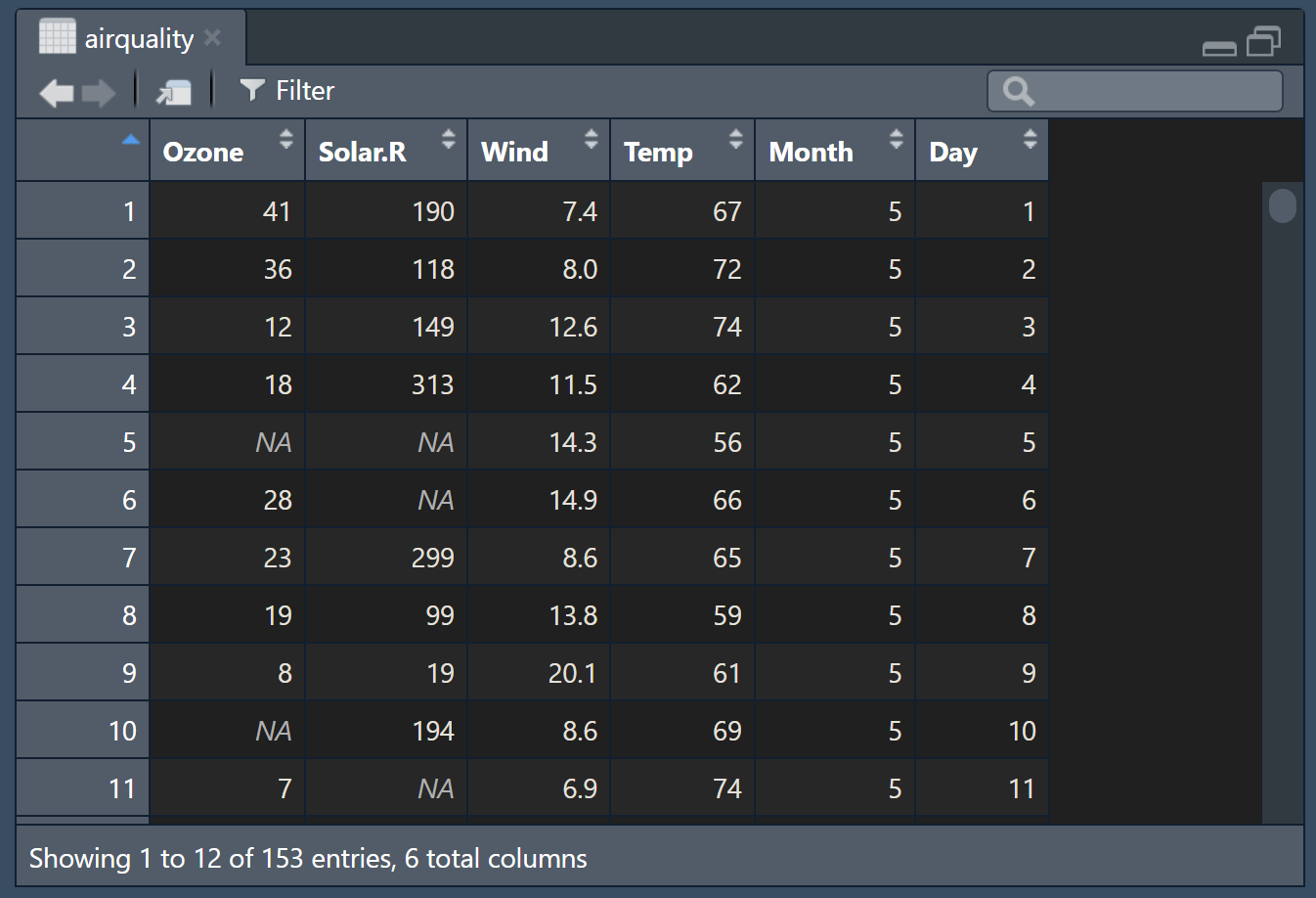

Figure A.1: Airquality Data Frame Preview in RStudio

str(airquality) # Display the structure of the dataset

#> 'data.frame':    153 obs. of  6 variables:
#>  $ Ozone  : int  41 36 12 18 NA 28 23 19 8 NA ...
#>  $ Solar.R: int  190 118 149 313 NA NA 299 99 19 194 ...
#>  $ Wind   : num  7.4 8 12.6 11.5 14.3 14.9 8.6 13.8 20.1 8.6 ...
#>  $ Temp   : int  67 72 74 62 56 66 65 59 61 69 ...
#>  $ Month  : int  5 5 5 5 5 5 5 5 5 5 ...
#>  $ Day    : int  1 2 3 4 5 6 7 8 9 10 ...

summary(airquality) # Gives summary statistics for each column

#>      Ozone           Solar.R           Wind             Temp      
#>  Min.   :  1.00   Min.   :  7.0   Min.   : 1.700   Min.   :56.00  
#>  1st Qu.: 18.00   1st Qu.:115.8   1st Qu.: 7.400   1st Qu.:72.00  
#>  Median : 31.50   Median :205.0   Median : 9.700   Median :79.00  
#>  Mean   : 42.13   Mean   :185.9   Mean   : 9.958   Mean   :77.88  
#>  3rd Qu.: 63.25   3rd Qu.:258.8   3rd Qu.:11.500   3rd Qu.:85.00  
#>  Max.   :168.00   Max.   :334.0   Max.   :20.700   Max.   :97.00  
#>  NA's   :37       NA's   :7                                       
#>      Month            Day      
#>  Min.   :5.000   Min.   : 1.0  
#>  1st Qu.:6.000   1st Qu.: 8.0  
#>  Median :7.000   Median :16.0  
#>  Mean   :6.993   Mean   :15.8  
#>  3rd Qu.:8.000   3rd Qu.:23.0  
#>  Max.   :9.000   Max.   :31.0  
#> 

#|
# 2. Select the first three columns (columns 1, 2, and 3)
airquality[, 1:3]

#>   Ozone Solar.R Wind
#> 1    41     190  7.4
#> 2    36     118  8.0
#> 3    12     149 12.6
#> 4    18     313 11.5
#> 5    NA      NA 14.3
#> 6    28      NA 14.9

Note

For clarity and conciseness, we have shortened the output to include only six rows.

# 3. Select rows 1 to 3, and columns 1 and 3
airquality[1:3, c(1, 3)]

#>   Ozone Wind
#> 1    41  7.4
#> 2    36  8.0
#> 3    12 12.6

# 4. Select rows 1 to 5, and column 1
airquality[1:5, 1]

#> [1] 41 36 12 18 NA

# 5. Select the first row
airquality[1, ]

#>   Ozone Solar.R Wind Temp Month Day
#> 1    41     190  7.4   67     5   1

# 6. Select the first 6 rows
airquality[1:6, ]

#>   Ozone Solar.R Wind Temp Month Day
#> 1    41     190  7.4   67     5   1
#> 2    36     118  8.0   72     5   2
#> 3    12     149 12.6   74     5   3
#> 4    18     313 11.5   62     5   4
#> 5    NA      NA 14.3   56     5   5
#> 6    28      NA 14.9   66     5   6

Return to Exercise 2.3.1

Solution 2.2.3: Matrix Operations

# Sales data (units sold)

sales_data <- c(500, 600, 550, 450, 620, 580, 610, 490, 530, 610, 570, 480)

# Create a matrix

sales_matrix <- matrix(sales_data, nrow = 4, ncol = 3, byrow = TRUE)

colnames(sales_matrix) <- c("Product_A", "Product_B", "Product_C")

rownames(sales_matrix) <- c("Region_1", "Region_2", "Region_3", "Region_4")

sales_matrix

#>          Product_A Product_B Product_C
#> Region_1       500       600       550
#> Region_2       450       620       580
#> Region_3       610       490       530
#> Region_4       610       570       480

# Task 1: Total units sold per product
total_units_per_product <- colSums(sales_matrix)

total_units_per_product

#> Product_A Product_B Product_C 
#>      2170      2280      2140

# Task 2: Average units sold for Product_A
average_product_a <- mean(sales_matrix[, "Product_A"])
average_product_a

#> [1] 542.5

# Task 3: Region with highest sales for Product_C
max_sales_product_c <- max(sales_matrix[, "Product_C"])
region_highest_sales <- rownames(sales_matrix)[which(sales_matrix[, "Product_C"] == max_sales_product_c)]
region_highest_sales # Returns the region name

#> [1] "Region_2"

Return to Exercise 2.2.3

Solution Quiz 2.3

Question 1:

Which function would you use to view the structure of a data frame, including its data types and a preview of its contents?

1. head()
   
2. str() ✓
   
3. summary()
   
4. names()

Question 2:

How do you access the third row and second column of a data frame df?

1. df[3, 2] ✓
   
2. df[[3, 2]]
   
3. df$3$2
   
4. df(3, 2)

Question 3:

In a data frame, all columns must contain the same type of data.

1. True

2. False ✓
   

Question 4:

Which of the following commands would open a spreadsheet-style viewer of the data frame df in RStudio?

1. View(df) ✓
   
2. view(df)
   
3. inspect(df)
   
4. display(df)

Question 5:

What does the summary() function provide when applied to a data frame?

1. Only the first few rows of the data frame.
   
2. Descriptive statistics for each column. ✓
   
3. The structure of the data frame including data types.
   
4. A visual plot of the data.

Answer: B

Question 6:

In a data frame, all columns must be of the same data type.

1. True

2. False ✓
   

Return to Quiz 2.3

Solution 2.3.2: Data Frame Manipulation

# Sample sales transactions
transaction_id <- 1:5

product <- c("Product_A", "Product_B", "Product_C", "Product_A", "Product_B")

quantity <- c(2, 5, 1, 3, 4)

price <- c(19.99, 5.49, 12.89, 19.99, 5.49)

total_amount <- quantity * price

sales_transactions <- data.frame(transaction_id, product, quantity, price, total_amount)

sales_transactions

#>   transaction_id   product quantity price total_amount
#> 1              1 Product_A        2 19.99        39.98
#> 2              2 Product_B        5  5.49        27.45
#> 3              3 Product_C        1 12.89        12.89
#> 4              4 Product_A        3 19.99        59.97
#> 5              5 Product_B        4  5.49        21.96

# Task 1: Add 'discounted_price' column
sales_transactions$discounted_price <- sales_transactions$price * 0.9
sales_transactions

#>   transaction_id   product quantity price total_amount discounted_price
#> 1              1 Product_A        2 19.99        39.98           17.991
#> 2              2 Product_B        5  5.49        27.45            4.941
#> 3              3 Product_C        1 12.89        12.89           11.601
#> 4              4 Product_A        3 19.99        59.97           17.991
#> 5              5 Product_B        4  5.49        21.96            4.941

# Task 2: Filter transactions with 'total_amount' > $50
high_value_transactions <- sales_transactions[sales_transactions$total_amount > 50, ]
high_value_transactions

#>   transaction_id   product quantity price total_amount discounted_price
#> 4              4 Product_A        3 19.99        59.97           17.991

# Task 3: Average 'total_amount' for 'Product_B'
product_b_transactions <- sales_transactions[sales_transactions$product == "Product_B", ]
average_total_amount_b <- mean(product_b_transactions$total_amount)
average_total_amount_b

#> [1] 24.705

Return to Exercise 2.3.2

Solution Quiz 2.4

Question 1:

Which function is used to create a list in R?

1. c()
   
2. list() ✓
   
3. data.frame()
   
4. matrix()

Question 2:

Given the list:

L <- list(a = 1, b = "text", c = TRUE)

how would you access the element "text"?

1. L[2]
   
2. L["b"]
   
3. L$b
   
4. Both b) and c) ✓
   

Question 3:

Using single square brackets [] to access elements in a list returns the element itself, not a sublist.

1. True

2. False ✓
   

Using single [] returns a sublist, while double [[ ]] returns the element itself.

Question 4:

How can you add a new element named d with value 3.14 to the list L?

1. L$d <- 3.14
   
2. L["d"] <- 3.14
   
3. L <- c(L, d = 3.14)
   
4. All of the above ✓

Question 5:

What will be the result of length(L) if

L <- list(a = 1, b = "text", c = TRUE, d = 3.14)?

1. 3
   
2. 4 ✓
   
3. 1
   
4. 0

Return to Quiz 2.4

Solution 2.4.1: Working with Lists

# Create the list
product_details <- list(
  product_id = 501,
  name = "Wireless Mouse",
  specifications = list(
    color = "Black",
    battery_life = "12 months",
    connectivity = "Bluetooth"
  ),
  in_stock = TRUE
)

# Access elements
product_details$product_id

#> [1] 501

product_details$name

#> [1] "Wireless Mouse"

product_details$in_stock

#> [1] TRUE

# Access nested list
product_details$specifications$color

#> [1] "Black"

product_details$specifications$connectivity

#> [1] "Bluetooth"

Return to Exercise 2.4.1

General Solution Quiz 2

Question 1

Which function is used to create a vector in R?

1. vector()
   
2. c() ✓
   
3. list()
   
4. data.frame()

Question 2

Which function is used to create a matrix in R?

1. array()
   
2. list()
   
3. matrix() ✓
   
4. data.frame()

Question 3

Which function is used to create an array in R?

1. list()
   
2. matrix()
   
3. c()
   
4. array() ✓
   

Question 4

Which function is used to create a list in R?

1. list() ✓
   
2. c()
   
3. matrix()
   
4. data.frame()

Question 5

A matrix in R must contain elements of:

1. Multiple data types (e.g., numeric and character mixed)
   
2. Only character type
   
3. Only logical type
   
4. The same type (all numeric, all logical, etc.) ✓
   

Question 6

An array in R can be:

1. Only two-dimensional
   
2. Only one-dimensional
   
3. Two-dimensional or higher ✓
   
4. Unlimited in one dimension only

Question 7

A list in R is considered:

1. Two-dimensional
   
2. One-dimensional ✓
   
3. Multi-dimensional
   
4. A type of matrix

Question 8

Which of the following is true about a list?

1. It can only contain numeric data
   
2. It stores data with rows and columns by default
   
3. It can store multiple data types in different elements ✓
   
4. It must be strictly two-dimensional

Question 9

What is the most suitable structure for storing heterogeneous data (e.g., numbers, characters, and even another data frame) in a single R object?

1. Vector
   
2. Matrix
   
3. Array
   
4. List ✓
   

Question 10

How do we typically check the “size” of a list in R?

1. nrow()
   
2. length() ✓
   
3. dim()
   
4. ncol()

Question 11

Which function is used to create a data frame in R?

1. data.frame() ✓
   
2. array()
   
3. c()
   
4. list()

Question 12

A data frame in R:

1. Must be strictly numeric
   
2. Can store different data types in each column ✓
   
3. Is always one-dimensional
   
4. Is identical to a matrix

Question 13

If you want to assign dimension names to an array, you should use:

1. rownames() only
   
2. colnames() only
   
3. dimnames() ✓
   
4. names()

Question 14

When creating a matrix using:

matrix(1:6, nrow = 2, ncol = 3, byrow = TRUE)

How are the elements placed?

1. Filled by columns first
   
2. Filled by rows first ✓
   
3. Randomly placed
   
4. Not possible to tell

Question 15

In an array with dimensions c(2, 3, 4), how many elements are there in total?

1. 12
   
2. 18
   
3. 24 ✓
   
4. 36

Return to General Quiz 2

Lab 3: Writing Custom Function

Solution 3.1.1: Temperature Conversion

celsius_to_fahrenheit <- function(celsius) {
  fahrenheit <- celsius * 1.8 + 32
  return(fahrenheit)
}

# Testing the function
celsius_to_fahrenheit(100)

#> [1] 212

celsius_to_fahrenheit(75)

#> [1] 167

celsius_to_fahrenheit(120)

#> [1] 248

Return to Exercise 3.1.1

Solution 3.1.2: Pythagoras Theorem

pythagoras <- function(a, b) {
  c <- sqrt(a^2 + b^2)
  return(c)
}

# Testing the function
pythagoras(3, 4)

#> [1] 5

pythagoras(4.1, 2.6)

#> [1] 4.854894

Return to Exercise 3.1.2

Solution 3.1.3: Staff Data Manipulation Using switch()

library(tidyverse)

#> ── Attaching core tidyverse packages ──────────────────────── tidyverse 2.0.0 ──
#> ✔ dplyr     1.1.4     ✔ readr     2.1.5
#> ✔ forcats   1.0.0     ✔ stringr   1.5.1
#> ✔ ggplot2   3.5.1     ✔ tibble    3.2.1
#> ✔ lubridate 1.9.3     ✔ tidyr     1.3.1
#> ✔ purrr     1.0.2     
#> ── Conflicts ────────────────────────────────────────── tidyverse_conflicts() ──
#> ✖ dplyr::filter() masks stats::filter()
#> ✖ dplyr::lag()    masks stats::lag()
#> ℹ Use the conflicted package (<http://conflicted.r-lib.org/>) to force all conflicts to become errors

# Sample employee data
staff_data <- data.frame(
  EmployeeID = 1:6,
  Name = c("Alice", "Ebunlomo", "Festus", "Othniel", "Bob", "Testimony"),
  Department = c("HR", "IT", "Finance", "Data Science", "Marketing", "Finance"),
  Salary = c(70000, 80000, 75000, 82000, 73000, 78000)
)

data_frame_operation <- function(data, operation) {
  result <- switch(operation,

    # Case 1: Summary of the data frame
    summary = {
      print("Summary of Data Frame:")
      summary(data)
    },

    # Case 2: Add a new column 'Bonus' which is 10% of the Salary
    add_column = {
      data$Bonus <- data$Salary * 0.10
      print("Data Frame after adding 'Bonus' column:")
      data
    },

    # Case 3: Filter employees with Salary > 75,000
    filter = {
      filtered_data <- filter(data, Salary > 75000)
      print("Filtered Data Frame (Salary > 75,000):")
      filtered_data
    },

    # Case 4: Group-wise average salary
    group_stats = {
      group_summary <- data %>%
        group_by(Department) %>%
        summarize(Average_Salary = mean(Salary))
      print("Group-wise Average Salary:")
      group_summary
    },

    # Case 5: Add a new column 'raise_salary' which is 5% of the Salary
    raise_salary = {
      data$Salary <- data$Salary * 1.05
      print("Data Frame after 5% salary increase:")
      data
    },

    # Default case
    {
      print("Invalid operation. Please choose a valid option.")
      NULL
    }
  )

  return(result)
}

# Testing the new operation
data_frame_operation(staff_data, "raise_salary")

#> [1] "Data Frame after 5% salary increase:"

#>   EmployeeID      Name   Department Salary
#> 1          1     Alice           HR  73500
#> 2          2  Ebunlomo           IT  84000
#> 3          3    Festus      Finance  78750
#> 4          4   Othniel Data Science  86100
#> 5          5       Bob    Marketing  76650
#> 6          6 Testimony      Finance  81900

Return to Exercise 3.1.3

Solution Quiz 3.1

Question 1:

What is the correct way to define a function in R?

1. function_name <- function { ... }

2. function_name <- function(...) { ... } ✓

3. function_name <- function[ ... ] { ... }

4. function_name <- function(...) [ ... ]

Question 2:

A variable defined inside a function is accessible outside the function.

1. True

2. False ✓
   

Question 3:

Which of the following is NOT a benefit of writing functions?

1. Code Reusability

2. Improved Readability

3. Increased Code Complexity ✓

4. Modular Programming

Return to Quiz 3.1

Lab 4: Managing Packages and Workflows

Solution Quiz 4.1

Question 1:

Imagine that you want to install the shiny package from CRAN. Which command should you use?

1. install.packages("shiny") ✓
   
2. library("shiny")
   
3. install.packages(shiny)
   
4. require("shiny")

Question 2:

What must you do after installing a package before you can use it in your current session?

1. Restart R
   
2. Run install.packages() again
   
3. Load it with library() ✓
   
4. Convert the package into a dataset

Question 3:

If you want to install a package that is not on CRAN (e.g., from GitHub), which additional package would be helpful?

1. installer
   
2. rio
   
3. devtools ✓
   
4. github_install

Question 4:

Which function would you use to update all outdated packages in your R environment?

1. update.packages() ✓
   
2. install.packages()
   
3. library()
   
4. require()

Question 5:

Which function can be used to check the version of an installed package?

1. version()
   
2. packageVersion() ✓
   
3. libraryVersion()
   
4. install.packages()

Return to Exercise 4.1

Solution Quiz 4.2

Question 1:

What is a key advantage of using RStudio Projects?

1. They automatically install packages.
   
2. They allow you to use absolute paths easily.
   
3. They set the working directory to the project folder, enabling relative paths. ✓
   
4. They prevent package updates.

Question 2:

Which file extension identifies an RStudio Project file?

1. .Rdata
   
2. .Rproj ✓
   
3. .Rmd
   
4. .Rscript

Question 3:

Why are relative paths preferable in a collaborative environment?

1. They are shorter and easier to type.
   
2. They change automatically when you move files.
   
3. They ensure that the code works regardless of the user’s file system structure. ✓
   
4. They are required for Git version control.

Return to Quiz 4.2

Solution Quiz 4.3

Question 1:

Which package is commonly used to read CSV files into R as tibbles?

1. readxl
   
2. haven
   
3. readr ✓
   
4. writexl

Question 2:

If you need to import an Excel file, which function would you likely use?

1. read_csv()
   
2. read_xlsx() ✓
   
3. read_sav()
   
4. read_dta()

Question 3:

Which package would you use to easily handle a wide variety of data formats without memorising specific functions for each?

1. rio ✓
   
2. haven
   
3. janitor
   
4. readxl

Question 4:

After cleaning and analysing your data, which function would you use to write the results to a CSV file?

1. write_xlsx()
   
2. exporter()
   
3. write_csv() ✓
   
4. import()

Return to Quiz 4.3

Lab 5: Data Transformation

Solution Quiz 5.1

Question 1:

What is the primary purpose of the pipe operator (|> or %>%) in R?

1. To run code in parallel.
   
2. To nest functions inside one another.
   
3. To pass the output of one function as the input to the next, improving code readability. ✓
   
4. To automatically clean missing data.

Question 2:

Consider the following R code snippets:

numbers <- c(2, 4, 6)

# Nested function version:
result1 <- round(sqrt(sum(numbers)))

# Pipe operator version:
result2 <- numbers |> sum() |> sqrt() |> round()

For a new R learner, is the pipe operator version generally more readable than the nested function version?

1. True ✓
   
2. False

Question 3:

What is the output of the following R code?

result <- c(5, 10, 15) 
result |> mean()

1. 10 ✓
   
2. 15
   
3. 5
   
4. 30

Question 4:

Which of the following code snippets correctly uses the pipe operator to apply the sqrt() function to the sum of numbers from 1 to 4?

1. sqrt(sum(1:4))
   
2. 1:4 |> sum() |> sqrt() ✓
   
3. sum(1:4) |> sqrt
   
4. 1:4 |> sqrt() |> sum()

Question 5:

What will be the output of the following code?

result <- letters
result |> head(3)

1. c("a", "b", "c") ✓
   
2. c("x", "y", "z")
   
3. c("A", "B", "C")
   
4. An error is thrown.

Return to Quiz 5.1

Solution Quiz 5.2

Question 1:

Which function would you use in dplyr to randomly select a specified number of rows from a dataset?

1. sample(n = 5)
   
2. slice_sample(n = 5) ✓
   
3. filter_sample()
   
4. mutate_sample()

Question 2:

To calculate the average sleep_total for each vore category, which combination of functions is most appropriate?

1. group_by(vore) |> select(sleep_total) |> summarise(mean(sleep_total))

2. select(vore, sleep_total) |> summarise(mean(sleep_total)) |> group_by(vore)

3. group_by(vore) |> summarise(avg_sleep = mean(sleep_total, na.rm = TRUE)) ✓
   

4. filter(vore) |> mutate(avg_sleep = mean(sleep_total))

Question 3:

To extract rows with the maximum value of a specified variable, which function is appropriate in dplyr?

1. slice_max() ✓
   
2. slice_min()
   
3. mutate()
   
4. select()

Question 4:

Which dplyr function would you use if you want to create a new column called weight_ratio by dividing bodywt by mean_bodywt?

1. filter()
   
2. select()
   
3. mutate() ✓
   
4. arrange()

Question 5:

Suppose you need to identify the top 3 penguins with the highest bill aspect ratio from the penguins dataset after calculating it in a new column. Which of the following code snippets is the most concise and appropriate?

penguins |>
  mutate(bill_aspect_ratio = bill_length_mm / bill_depth_mm) |>
  arrange(desc(bill_aspect_ratio)) |>
  head(3)

penguins |>
  mutate(bill_aspect_ratio = bill_length_mm / bill_depth_mm) |>
  slice_max(bill_aspect_ratio, n = 3)

3. Both a and b are equally concise and valid. ✓
   

4. Neither a nor b is valid.

Question 6:

Given the following code, which is the correct equivalent using the pipe operator?

result <- arrange(filter(select(msleep, name, sleep_total), sleep_total > 8), sleep_total)

1. msleep |> select(name, sleep_total) |> filter(sleep_total > 8) |> arrange(sleep_total) ✓

2. msleep |> filter(sleep_total > 8) |> select(name, sleep_total) |> arrange(sleep_total)

3. select(msleep, name, sleep_total) |> filter(sleep_total > 8) |> arrange(sleep_total)

4. msleep |> arrange(sleep_total) |> filter(sleep_total > 8) |> select(name, sleep_total)

Question 7:

Which of the following correctly applies a log transformation to numeric columns only?

mutate_all(log)

mutate(across(everything(), log))

mutate(select(where(is.numeric), log))

4. ✓
   

mutate(across(where(is.numeric), log))

Question 8:

What does mutate(across(everything(), as.character)) do?

1. Converts all character columns to numeric.
   
2. Converts all columns in the dataset to character type. ✓
   
3. Applies a conditional transformation to numeric columns.
   
4. Filters out non-character values.

Question 9:

To extract the rows with the minimum value of a specified variable, which dplyr function should you use?

1. slice_min() ✓
   
2. slice_max()
   
3. arrange()
   
4. filter()

Question 10:

If you want to reorder the rows of msleep by sleep_total in ascending order and then only show the top 5 rows, which code snippet is correct?

1. msleep |> arrange(sleep_total) |> head(5) ✓

2. msleep |> head(5) |> arrange(sleep_total)

3. msleep |> summarise(sleep_total) |> head(5)

4. msleep |> select(sleep_total) |> arrange(desc(sleep_total)) |> head(5)

Return to Quiz 5.2

Solution 5.2.1: Top 5 Carnivorous Animals

msleep |>
  filter(vore == "carni") |>
  mutate(sleep_to_weight = sleep_total / bodywt) |>
  select(name, sleep_total, sleep_to_weight) |>
  slice_max(sleep_total, n = 5)

#> # A tibble: 5 × 3
#>   name                       sleep_total sleep_to_weight
#>   <chr>                            <dbl>           <dbl>
#> 1 Thick-tailed opposum              19.4         52.4   
#> 2 Long-nosed armadillo              17.4          4.97  
#> 3 Tiger                             15.8          0.0972
#> 4 Northern grasshopper mouse        14.5        518.    
#> 5 Lion                              13.5          0.0836

Return to Exercise 5.2.1

Solution Quiz 5.3

Question 1:

Which function in R checks if there are any missing values in an object?

1. is.na()
   
2. anyNA() ✓
   
3. complete.cases()
   
4. na.omit()

Question 2:

Which approach removes any rows containing NA values?

1. na.omit() ✓
   
2. replace_na()
   
3. complete.cases()
   
4. anyNA()

Question 3:

If you decide to impute missing values in a column using the median, what is one potential advantage of using the median rather than the mean?

1. The median is always easier to compute.
   
2. The median is more affected by outliers than the mean.
   
3. The median is less influenced by extreme values and may provide a more robust estimate. ✓
   
4. The median will always be exactly halfway between the min and max values.

Question 4:

How would you replace all NA values in character columns with "Unknown"?

1. ✓
   

mutate(across(where(is.character), ~ replace_na(., "Unknown")))

mutate_all(~ replace_na(., "Unknown"))

mutate(across(where(is.character), na.omit))

mutate(across(where(is.character), replace(. == NA, "Unknown")))

Question 5:

What does the anyNA() function return?

1. The number of missing values in an object.
   
2. TRUE if there are any missing values in the object; otherwise, FALSE. ✓
   
3. A logical vector of missing values in each row.
   
4. A subset of the data frame without missing values.

Question 6:

You want to create a new column in a data frame that flags rows with missing values as TRUE. Which code achieves this?

1. df$new_col <- !complete.cases(df) ✓
   
2. df$new_col <- complete.cases(df)
   
3. df$new_col <- anyNA(df)
   
4. df$new_col <- is.na(df)

Question 7:

Before removing rows with missing values, what is an important consideration?

1. Whether the missing values are randomly distributed across the data. ✓
   
2. Whether the dataset is stored in a data frame.
   
3. Whether missing values exist in every column.
   
4. Whether the missing values are encoded as NA.

Question 8:

Why should the proportion of missing data in a row or column be considered before removing it?

1. Removing rows or columns with minimal missing values may lead to excessive data loss. ✓
2. Columns with missing values cannot be visualized.
3. Rows with missing values are always irrelevant.
4. Rows with missing values should never be analysed.

Question 9:

If a dataset has 50% missing values in a column, what is a common approach to handle this situation?

1. Replace missing values with the column mean.
   
2. Remove the column entirely. ✓
   
3. Replace missing values with zeros.
   
4. Leave the missing values as they are.

Question 10:

What does the following Tidyverse-style code do?

library(dplyr)

airquality_data <- airquality_data %>%
  mutate(Ozone = if_else(is.na(Ozone), mean(Ozone, na.rm = TRUE), Ozone))

1. Removes rows where Ozone is missing.
   
2. Replaces missing values in Ozone with the mean of the column. ✓
   
3. Flags rows where Ozone is missing.
   
4. Deletes the Ozone column if it has missing values.

Return to Quiz 5.3

Solution 5.3.1: Missing Data Analysis Report for the Television Company Dataset

In this report, we explore several methods for dealing with missing data in a television company dataset. First, we import the data, then apply four different approaches to address any missing values. After evaluating the results, we conclude with a recommendation on the best method to use.

Data Import & Initial Inspection

We begin by loading the dataset and inspecting its structure, summary statistics, and missing values.

library(tidyverse)

# Import the dataset
tv_data <- read_csv("r-data/data-tv-company.csv")

# Inspect the data structure and summary statistics
glimpse(tv_data)

#> Rows: 462
#> Columns: 9
#> $ regard  <dbl> 8, 5, 5, 4, 6, 6, 4, 5, 7, NA, 6, 5, 5, 3, 4, 5, 5, NA, 5, 7, …
#> $ gender  <chr> "Male", "Female", "Female", "Female", "Female", "Female", "Fem…
#> $ views   <dbl> 458, 460, 457, 437, 438, 456, NA, 448, 450, 459, 442, 443, 451…
#> $ online  <dbl> 821, 810, 824, 803, 791, 813, 797, 813, 827, 820, 802, 812, 81…
#> $ library <dbl> 104, 99, NA, NA, 84, 104, NA, 94, 100, 103, 101, 90, 99, 94, 9…
#> $ Show1   <dbl> 74, 70, 72, 74, 74, 73, 71, 73, 79, 77, 70, 74, 73, 72, 71, 78…
#> $ Show2   <dbl> 74, 74, 72, 74, 70, 73, 71, 72, 76, 77, 69, 70, 72, 73, 70, 76…
#> $ Show3   <dbl> 64, 58, 59, 58, 57, 61, 58, 58, 62, 60, 62, 59, 59, 58, 58, 60…
#> $ Show4   <dbl> 39, 44, 34, 39, 34, 40, 40, 31, 44, 35, 37, 33, 36, 35, 37, 37…

summary(tv_data)

#>      regard         gender              views           online   
#>  Min.   :2.000   Length:462         Min.   :430.0   Min.   :787  
#>  1st Qu.:5.000   Class :character   1st Qu.:445.0   1st Qu.:809  
#>  Median :5.000   Mode  :character   Median :450.0   Median :815  
#>  Mean   :5.454                      Mean   :449.9   Mean   :815  
#>  3rd Qu.:6.000                      3rd Qu.:456.0   3rd Qu.:821  
#>  Max.   :9.000                      Max.   :474.0   Max.   :843  
#>  NA's   :30                         NA's   :22                   
#>     library           Show1           Show2           Show3      
#>  Min.   : 84.00   Min.   :66.00   Min.   :64.00   Min.   :55.00  
#>  1st Qu.: 95.00   1st Qu.:72.00   1st Qu.:71.00   1st Qu.:59.00  
#>  Median : 98.00   Median :73.00   Median :72.00   Median :60.00  
#>  Mean   : 98.14   Mean   :73.08   Mean   :72.16   Mean   :59.87  
#>  3rd Qu.:101.00   3rd Qu.:75.00   3rd Qu.:74.00   3rd Qu.:61.00  
#>  Max.   :115.00   Max.   :79.00   Max.   :78.00   Max.   :66.00  
#>  NA's   :68                                                      
#>      Show4      
#>  Min.   :21.00  
#>  1st Qu.:34.00  
#>  Median :37.00  
#>  Mean   :37.42  
#>  3rd Qu.:41.00  
#>  Max.   :50.00  
#> 

# Count missing values per row
count_missing_rows <- function(data) {
  sum(apply(data, MARGIN = 1, function(x) any(is.na(x))))
}

count_missing_rows(tv_data)

#> [1] 112

Tip

apply(data, MARGIN = 1, function(x) any(is.na(x))):

• MARGIN = 1: Instructs apply() to iterate over rows of the data frame (if set to 2, it would iterate over columns).

• function(x) any(is.na(x)): For each row, checks if any element is missing (i.e., is NA), returning TRUE if so.

sum(...):

• Sums the logical vector produced by apply(), where each TRUE is counted as 1, thereby giving the total number of rows with at least one missing value.

# Count missing values per column using inspectdf
tv_data %>%
  inspectdf::inspect_na()

#> # A tibble: 9 × 3
#>   col_name   cnt  pcnt
#>   <chr>    <int> <dbl>
#> 1 library     68 14.7 
#> 2 regard      30  6.49
#> 3 views       22  4.76
#> 4 gender       0  0   
#> 5 online       0  0   
#> 6 Show1        0  0   
#> 7 Show2        0  0   
#> 8 Show3        0  0   
#> 9 Show4        0  0

Strategies for Dealing with Missing Data

Below, we demonstrate four different methods to handle missing data in the dataset.

Method 1: Complete Case Analysis

Remove all rows with any missing values.

tv_data_complete <- tv_data %>% drop_na()

Tip

Alternatively, you can use na.omit() to remove rows with missing values:

tv_data %>% na.omit()

#> # A tibble: 350 × 9
#>    regard gender views online library Show1 Show2 Show3 Show4
#>     <dbl> <chr>  <dbl>  <dbl>   <dbl> <dbl> <dbl> <dbl> <dbl>
#>  1      8 Male     458    821     104    74    74    64    39
#>  2      5 Female   460    810      99    70    74    58    44
#>  3      6 Female   438    791      84    74    70    57    34
#>  4      6 Female   456    813     104    73    73    61    40
#>  5      5 Male     448    813      94    73    72    58    31
#>  6      7 Female   450    827     100    79    76    62    44
#>  7      6 Female   442    802     101    70    69    62    37
#>  8      5 Female   443    812      90    74    70    59    33
#>  9      5 Female   451    815      99    73    72    59    36
#> 10      3 Male     440    810      94    72    73    58    35
#> # ℹ 340 more rows

Method 2: Numeric Imputation with Column Means

Replace missing values in all numeric columns with the respective column mean.

tv_data_mean_imputed <- tv_data %>%
  bulkreadr::fill_missing_values(method = "mean")

Method 3: Targeted Replacement using tidyr::replace_na() with Medians

For numeric columns with missing values (regard, views, and library), replace NAs with the column median.

tv_data_tidyr <- tv_data %>%
  replace_na(list(
    regard  = median(tv_data$regard, na.rm = TRUE),
    views   = median(tv_data$views, na.rm = TRUE),
    library = median(tv_data$library, na.rm = TRUE)
  ))

Tip

Alternatively, you can use the selected_variables argument in the bulkreadr::fill_missing_values() function with method = "median" to impute these missing values:

tv_data_mean_imputed <- tv_data %>%
  bulkreadr::fill_missing_values(selected_variables = c("regard", "views", "library"), method = "median")

Evaluation and Selection

Based on the outputs from the various methods, here is a summary and evaluation of each approach:

Original Data:

• Dimensions: 462 rows × 9 columns.

• Missing Values:

  • regard: 30 missing
    
  • views: 22 missing
    
  • library: 68 missing

Complete Case Analysis:

• Dimensions: 350 rows × 9 columns.

• Summary: All rows with any missing values were removed, resulting in a loss of about 24% of the data.

• Consideration: Although this method produces a dataset free of missing values, it may discard valuable information and reduce the statistical power of subsequent analyses.

Numeric Imputation (Replacing Missing Numeric Values with Column Means):

• Dimensions: 462 rows × 9 columns.

• Summary: Missing numeric values in columns such as regard, views, and library have been replaced by their respective column means. The summary no longer shows missing value counts for these columns.

• Consideration: This method preserves all observations but may smooth out natural variability, potentially impacting the distribution and variance in the data.

Targeted Replacement using tidyr::replace_na():

• Dimensions: 462 rows × 9 columns.

• Summary: Missing values in numeric columns (regard, views, library) have been replaced by their respective medians, resulting in a dataset identical in dimensions to the original but with imputed values.

• Consideration: This method retains the full dataset and provides robust imputation for numeric data, preserving the distribution better than mean imputation.

Conclusion

In summary, after comparing the different approaches:

• Complete Case Analysis yields a clean dataset but reduces the sample size.

• Numeric Imputation retains all data by substituting missing values with means, although it may reduce variability.

• Targeted Replacement (using medians) preserves the full dataset and is robust to outliers.

Recommendation:

Method 3 (Targeted Replacement using Medians) is preferred because it maintains the full dataset while providing robust imputation for missing numeric values.

Return to Exercise 5.3.1

Lab 6: Tidy Data and Joins

Solution Quiz 6.1

Question 1:

Consider the following data frame:

sales_data_wide <- data.frame(
  Month = c("Oct", "Nov", "Dec"),
  North = c(180, 190, 200),
  East  = c(177, 183, 190),
  South = c(150, 140, 160),
  West  = c(200, 220, 210)
)

Which function would you use to convert this wide-format dataset into a long-format dataset?

1. pivot_long()
   
2. pivot_wider()
   
3. separate()
   
4. pivot_longer() ✓
   

Question 2:

In the pivot_longer() function, if you want the original column names (“North”, “East”, “South”, “West”) to appear in a new column called “Region”, which argument would you use?

1. cols
   
2. names_to ✓
   
3. values_to
   
4. names_prefix

Question 3:

Given the same data frame, which argument in pivot_longer() specifies the name of the new column that stores the sales figures?

1. names_to
   
2. values_to ✓
   
3. cols
   
4. values_drop_na

Question 4:

What is the primary purpose of using pivot_wider()?

1. To convert long-format data into wide format ✓
   
2. To combine two data frames
   
3. To split a column into multiple columns
   
4. To remove missing values

Question 5:

If you apply pivot_longer() on sales_data_wide without specifying cols, what is likely to happen?

1. All columns will be pivoted, including the identifier column “Month”, leading to an undesired result. ✓
   
2. Only numeric columns will be pivoted.
   
3. The function will automatically ignore non-numeric columns.
   
4. An error will be thrown immediately.

Question 6:

Which package provides the functions pivot_longer() and pivot_wider()?

1. dplyr
   
2. tidyr ✓
   
3. ggplot2
   
4. readr

Question 7:

The functions pivot_longer() and pivot_wider() are inverses of each other, allowing you to switch between wide and long formats easily.

1. True ✓
   
2. False

Question 8:

In the following code snippet, what is the role of the cols = c(North, East, South, West) argument?

sales_data_long <- sales_data_wide |> 
  pivot_longer(
    cols = c(North, East, South, West), 
    names_to = "Region", 
    values_to = "Sales"
  )

1. It tells pivot_longer() which columns to keep as they are.
   
2. It specifies the columns to be pivoted from wide to long format. ✓
   
3. It defines the new column names for the output.
   
4. It removes missing values from these columns.

Question 9:

After reshaping the data to long format, which of the following is a potential advantage?

1. Easier to merge with other datasets
   
2. Simplified time series analysis and visualisation ✓
   
3. Increased redundancy in the dataset
   
4. Reduced number of observations

Question 10:

Which of the following best describes tidy data?

1. Each variable forms a column and each observation a row ✓
   
2. Data is merged from multiple sources
   
3. Data is automatically plotted
   
4. Missing values are always removed

Return to Quiz 6.1

Solution 6.1.1: Tidying the Pew Religion and Income Survey Data

In this solution, we tidy the religion_income dataset from the Pew Research Trust’s 2014 survey. The dataset includes one column for religion and multiple columns for various income ranges (e.g., <$10k, $10-20k, $20-30k, etc.), each indicating the number of respondents who fall within that bracket. Our goals are:

1. Import and Inspect the data.

2. Reshape the dataset from wide to long format, gathering all income range columns into two new variables: income_range and respondents.

3. Create a Summary that shows the total number of respondents for each income range, sorted in a logical order.

4. Identify which religious affiliation has the highest number of respondents in the top income bracket (>150k).

5. Visualise the distribution of respondents by income range.

Importing and Inspecting the Data

We begin by loading the tidyverse package and importing the dataset from the r-data directory. We then use glimpse() to verify that the file has loaded correctly and to explore its structure.

library(tidyverse)

# Import the dataset
relig_income <- read_csv("r-data/religion-income.csv")

#> Rows: 18 Columns: 11
#> ── Column specification ────────────────────────────────────────────────────────
#> Delimiter: ","
#> chr  (1): religion
#> dbl (10): <$10k, $10-20k, $20-30k, $30-40k, $40-50k, $50-75k, $75-100k, $100...
#> 
#> ℹ Use `spec()` to retrieve the full column specification for this data.
#> ℹ Specify the column types or set `show_col_types = FALSE` to quiet this message.

# Inspect the data structure
glimpse(relig_income)

#> Rows: 18
#> Columns: 11
#> $ religion             <chr> "Agnostic", "Atheist", "Buddhist", "Catholic", "D…
#> $ `<$10k`              <dbl> 27, 12, 27, 418, 15, 575, 1, 228, 20, 19, 289, 29…
#> $ `$10-20k`            <dbl> 34, 27, 21, 617, 14, 869, 9, 244, 27, 19, 495, 40…
#> $ `$20-30k`            <dbl> 60, 37, 30, 732, 15, 1064, 7, 236, 24, 25, 619, 4…
#> $ `$30-40k`            <dbl> 81, 52, 34, 670, 11, 982, 9, 238, 24, 25, 655, 51…
#> $ `$40-50k`            <dbl> 76, 35, 33, 638, 10, 881, 11, 197, 21, 30, 651, 5…
#> $ `$50-75k`            <dbl> 137, 70, 58, 1116, 35, 1486, 34, 223, 30, 95, 110…
#> $ `$75-100k`           <dbl> 122, 73, 62, 949, 21, 949, 47, 131, 15, 69, 939, …
#> $ `$100-150k`          <dbl> 109, 59, 39, 792, 17, 723, 48, 81, 11, 87, 753, 4…
#> $ `>150k`              <dbl> 84, 74, 53, 633, 18, 414, 54, 78, 6, 151, 634, 42…
#> $ `Don't know/refused` <dbl> 96, 76, 54, 1489, 116, 1529, 37, 339, 37, 162, 13…

The religion income data is arranged in a compact or wide format. Each row represents a religious affiliation, and each income range column shows the number of respondents in that bracket.

Tidying the Data

We transform the data from wide to long format using pivot_longer(), gathering all columns except religion into two new columns: income_range (for the bracket names) and respondents (for the counts).

relig_income_long <- relig_income %>%
  pivot_longer(
    cols = -religion, # All columns except 'religion'
    names_to = "income_range", # New column for the original income range names
    values_to = "respondents" # New column for the corresponding counts
  )

# Inspect the tidied data
glimpse(relig_income_long)

#> Rows: 180
#> Columns: 3
#> $ religion     <chr> "Agnostic", "Agnostic", "Agnostic", "Agnostic", "Agnostic…
#> $ income_range <chr> "<$10k", "$10-20k", "$20-30k", "$30-40k", "$40-50k", "$50…
#> $ respondents  <dbl> 27, 34, 60, 81, 76, 137, 122, 109, 84, 96, 12, 27, 37, 52…

Each row now represents a unique combination of religion and income bracket, along with the corresponding number of respondents.

Creating a Summary Table

We group the tidied data by income_range and sum the total respondents. To achieve a logical order (lowest to highest income), we define a custom factor level, then arrange accordingly.

income_levels <- c(
  "<$10k",
  "$10-20k",
  "$20-30k",
  "$30-40k",
  "$40-50k",
  "$50-75k",
  "$75-100k",
  "$100-150k",
  ">150k",
  "Don't know/refused"
)

income_summary <- relig_income_long %>%
  mutate(income_range = factor(income_range, levels = income_levels)) %>%
  group_by(income_range) %>%
  summarise(total_respondents = sum(respondents, na.rm = TRUE)) %>%
  ungroup()

income_summary

#> # A tibble: 10 × 2
#>    income_range       total_respondents
#>    <fct>                          <dbl>
#>  1 <$10k                           1930
#>  2 $10-20k                         2781
#>  3 $20-30k                         3357
#>  4 $30-40k                         3302
#>  5 $40-50k                         3085
#>  6 $50-75k                         5185
#>  7 $75-100k                        3990
#>  8 $100-150k                       3197
#>  9 >150k                           2608
#> 10 Don't know/refused              6121

The data now shows the total number of respondents in each bracket, sorted from <$10k to >150k, with “Don’t know/refused” at the end.

Identifying Which Religion Has the Largest Number of Respondents in the >150k Bracket

We can now focus on the >150k bracket to see which religion leads in this top income category.

top_bracket <- relig_income_long %>%
  filter(income_range == ">150k") %>%
  group_by(religion) %>%
  summarise(total_in_top_bracket = sum(respondents, na.rm = TRUE)) %>%
  arrange(desc(total_in_top_bracket))

top_bracket

#> # A tibble: 18 × 2
#>    religion                total_in_top_bracket
#>    <chr>                                  <dbl>
#>  1 Mainline Prot                            634
#>  2 Catholic                                 633
#>  3 Evangelical Prot                         414
#>  4 Unaffiliated                             258
#>  5 Jewish                                   151
#>  6 Agnostic                                  84
#>  7 Historically Black Prot                   78
#>  8 Atheist                                   74
#>  9 Hindu                                     54
#> 10 Buddhist                                  53
#> 11 Orthodox                                  46
#> 12 Mormon                                    42
#> 13 Other Faiths                              41
#> 14 Don't know/refused                        18
#> 15 Other Christian                           12
#> 16 Jehovah's Witness                          6
#> 17 Muslim                                     6
#> 18 Other World Religions                      4

We see that Mainline Protestant affiliates have the greatest number of respondents in the >150k bracket (634), closely followed by Catholics (633).

Visualising the Distribution of Respondents by Income Range

Finally, we create a bar chart with numeric labels on each bar, making it easy to compare the total respondents across income brackets.

income_summary |>
  ggplot(aes(x = income_range, y = total_respondents, fill = income_range)) +
  geom_col(show.legend = FALSE) +
  geom_text(aes(label = total_respondents), vjust = -0.3, size = 3) +
  labs(
    title = "Total Respondents by Income Range",
    x = "Income Range",
    y = "Total Respondents"
  ) +
  theme_minimal() +
  theme(axis.text.x = element_text(angle = 45, hjust = 1))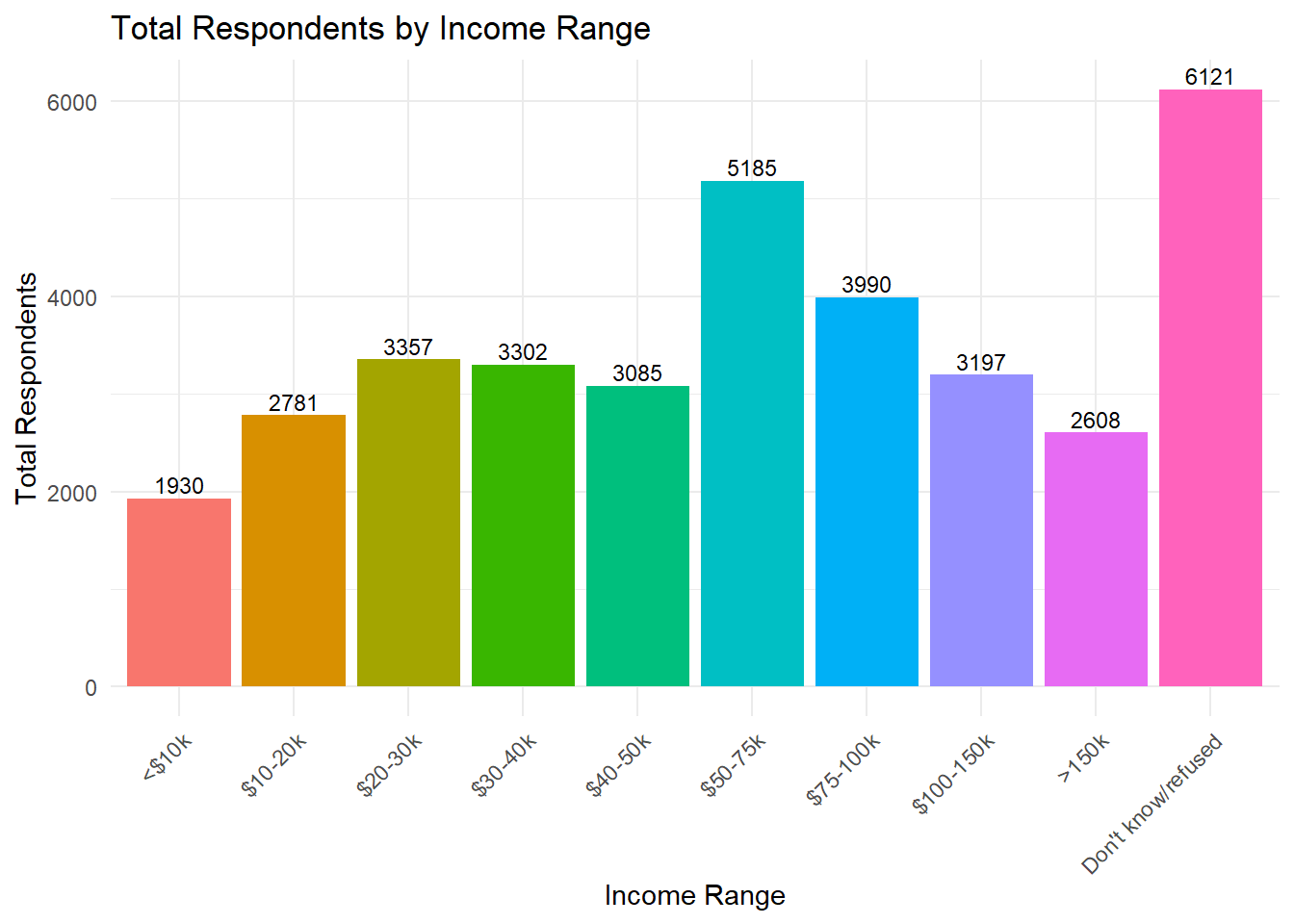

The bar chart shows each income bracket on the x-axis, with its total respondents on the y-axis. Each bar is labelled with the corresponding numeric value, offering a clear comparison. “Don’t know/refused” emerges as the largest category (6121), followed by $50-75k (5185).

Return to Exercise 6.1.1

Solution Quiz 6.2

Question 1:

Given the following tibble:

tb_cases <- tibble(
  country = c("Brazil", "Brazil", "China", "China"),
  year = c(1999, 2000, 1999, 2000),
  rate = c("37737/172006362", "80488/174504898", "212258/1272915272", "213766/1280428583")
)

Which function would you use to split the "rate" column into two separate columns for cases and population?

1. separate() ✓
   
2. unite()
   
3. pivot_longer()
   
4. pivot_wider()

Question 2:

Which argument in separate() allows automatic conversion of new columns to appropriate data types?

1. remove
   
2. auto
   
3. convert ✓
   
4. into

Question 3:

Which function would you use to merge two columns into one, for example, combining separate “century” and “year” columns?

1. separate()
   
2. unite() ✓
   
3. pivot_longer()
   
4. pivot_wider()

Question 4:

In the separate() function, what does the sep argument define?

1. The new column names
   
2. The delimiter at which to split the column ✓
   
3. The data frame to be merged
   
4. The columns to remove

Question 5:

Consider the following data frame:

tb_cases <- tibble(
  country = c("Afghanistan", "Brazil", "China"),
  century = c("19", "19", "19"),
  year = c("99", "99", "99")
)

Which code correctly combines “century” and “year” into a single column “year” without any separator?

1. tb_cases |> unite(year, century, year, sep = "") ✓

2. tb_cases |> separate(year, into = c("century", "year"), sep = "")

3. tb_cases |> unite(year, century, year, sep = "_")

4. tb_cases |> pivot_longer(cols = c(century, year))

Question 6:

When using separate(), how can you retain the original column after splitting it?

1. Set remove = FALSE ✓
   
2. Set convert = TRUE
   
3. Use unite() instead
   
4. Omit the sep argument

Question 7:

Which variant of separate() would you use to split a column at fixed character positions?

1. separate_wider_delim()
   
2. separate_wider_regex()
   
3. separate_wider_position() ✓
   
4. separate()

Question 8:

By default, the unite() function removes the original columns after combining them.

1. True ✓
   
2. False

Question 9:

What is the main benefit of using separate() on a column that combines multiple data points (e.g. “745/19987071”)?

1. It facilitates the conversion of string data into numeric data automatically.
   
2. It simplifies further analysis by splitting combined information into distinct, analysable components. ✓
   
3. It merges the data with another dataset.
   
4. It increases data redundancy.

Question 10:

Which argument in unite() determines the character inserted between values when combining columns?

1. separator
   
2. sep ✓
   
3. col
   
4. delimiter

Return to Quiz 6.2

Solution 6.2.1: Transforming the Television Company Dataset

In this solution, we will demonstrate how to clean and transform the television-company-data.csv dataset. Our primary goal is to split the combined Shows column into four separate columns (one for each show), calculate the average score across these shows, and then analyse these averages by gender.

Importing and Inspecting the Data

First, we import the dataset using read_csv() and inspect its structure using glimpse(). This helps us understand the data and verify that the file has been loaded correctly.

library(tidyverse)

# Import the dataset from the r-data directory
tv_data <- read_csv("r-data/television-company-data.csv")

# Inspect the data structure

tv_data

#> # A tibble: 462 × 6
#>    regard gender views online library Shows          
#>     <dbl> <chr>  <dbl>  <dbl>   <dbl> <chr>          
#>  1      8 Male     458    821     104 74,  74, 64, 39
#>  2      5 Female   460    810      99 70,  74, 58, 44
#>  3      5 Female   457    824      NA 72,  72, 59, 34
#>  4      4 Female   437    803      NA 74,  74, 58, 39
#>  5      6 Female   438    791      84 74,  70, 57, 34
#>  6      6 Female   456    813     104 73,  73, 61, 40
#>  7      4 Female    NA    797      NA 71,  71, 58, 40
#>  8      5 Male     448    813      94 73,  72, 58, 31
#>  9      7 Female   450    827     100 79,  76, 62, 44
#> 10     NA Female   459    820     103 77,  77, 60, 35
#> # ℹ 452 more rows

glimpse(tv_data)

#> Rows: 462
#> Columns: 6
#> $ regard  <dbl> 8, 5, 5, 4, 6, 6, 4, 5, 7, NA, 6, 5, 5, 3, 4, 5, 5, NA, 5, 7, …
#> $ gender  <chr> "Male", "Female", "Female", "Female", "Female", "Female", "Fem…
#> $ views   <dbl> 458, 460, 457, 437, 438, 456, NA, 448, 450, 459, 442, 443, 451…
#> $ online  <dbl> 821, 810, 824, 803, 791, 813, 797, 813, 827, 820, 802, 812, 81…
#> $ library <dbl> 104, 99, NA, NA, 84, 104, NA, 94, 100, 103, 101, 90, 99, 94, 9…
#> $ Shows   <chr> "74,  74, 64, 39", "70,  74, 58, 44", "72,  72, 59, 34", "74, …

The television company data contains 462 rows and 10 columns, including variables for viewer regard, gender, number of views, online interactions, library usage, and four show scores.

Splitting the ‘Shows’ Column

The Shows column contains scores for four different shows, separated by commas. We use the separate() function to split this column into four new columns named Show1, Show2, Show3, and Show4. The argument convert = TRUE automatically converts these new columns to numeric values, ensuring they are ready for analysis.

tv_data <- tv_data %>%
  separate(Shows,
    into = c("Show1", "Show2", "Show3", "Show4"),
    sep = ",",
    convert = TRUE
  )

# Check the transformed data
glimpse(tv_data)

#> Rows: 462
#> Columns: 9
#> $ regard  <dbl> 8, 5, 5, 4, 6, 6, 4, 5, 7, NA, 6, 5, 5, 3, 4, 5, 5, NA, 5, 7, …
#> $ gender  <chr> "Male", "Female", "Female", "Female", "Female", "Female", "Fem…
#> $ views   <dbl> 458, 460, 457, 437, 438, 456, NA, 448, 450, 459, 442, 443, 451…
#> $ online  <dbl> 821, 810, 824, 803, 791, 813, 797, 813, 827, 820, 802, 812, 81…
#> $ library <dbl> 104, 99, NA, NA, 84, 104, NA, 94, 100, 103, 101, 90, 99, 94, 9…
#> $ Show1   <int> 74, 70, 72, 74, 74, 73, 71, 73, 79, 77, 70, 74, 73, 72, 71, 78…
#> $ Show2   <int> 74, 74, 72, 74, 70, 73, 71, 72, 76, 77, 69, 70, 72, 73, 70, 76…
#> $ Show3   <int> 64, 58, 59, 58, 57, 61, 58, 58, 62, 60, 62, 59, 59, 58, 58, 60…
#> $ Show4   <int> 39, 44, 34, 39, 34, 40, 40, 31, 44, 35, 37, 33, 36, 35, 37, 37…

We now have separate columns (Show1, Show2, Show3, Show4) for each show’s score. The dataset still has 462 rows, but now includes 9 columns: the original variables plus the newly created show score columns and excluding variable Shows.

Calculating the Mean Show Score

Next, we create a new variable, mean_show, which represents the average score across the four shows. In this step, we use rowwise() along with mutate() to calculate the mean for each observation. The na.rm = TRUE argument ensures that any missing values are ignored during the calculation. After computing the mean, we use ungroup() to remove the row-wise grouping.

tv_data <- tv_data %>%
  rowwise() %>%
  mutate(mean_show = mean(c(Show1, Show2, Show3, Show4), na.rm = TRUE)) %>%
  ungroup()

# updated dataset with the new variable
tv_data

#> # A tibble: 462 × 10
#>    regard gender views online library Show1 Show2 Show3 Show4 mean_show
#>     <dbl> <chr>  <dbl>  <dbl>   <dbl> <int> <int> <int> <int>     <dbl>
#>  1      8 Male     458    821     104    74    74    64    39      62.8
#>  2      5 Female   460    810      99    70    74    58    44      61.5
#>  3      5 Female   457    824      NA    72    72    59    34      59.2
#>  4      4 Female   437    803      NA    74    74    58    39      61.2
#>  5      6 Female   438    791      84    74    70    57    34      58.8
#>  6      6 Female   456    813     104    73    73    61    40      61.8
#>  7      4 Female    NA    797      NA    71    71    58    40      60  
#>  8      5 Male     448    813      94    73    72    58    31      58.5
#>  9      7 Female   450    827     100    79    76    62    44      65.2
#> 10     NA Female   459    820     103    77    77    60    35      62.2
#> # ℹ 452 more rows

The dataset now includes an additional column, mean_show, which holds each viewer’s average score across the four shows.

Analysing the Data by Gender

To explore how viewer ratings differ by gender, we group the data by the gender variable and calculate the average mean_show for each group using group_by() and summarise(). We also count the number of observations per group.

gender_summary <- tv_data %>%
  group_by(gender) %>%
  summarise(
    mean_of_mean_show = mean(mean_show, na.rm = TRUE),
    count = n()
  )

# Display the summary
gender_summary

#> # A tibble: 3 × 3
#>   gender     mean_of_mean_show count
#>   <chr>                  <dbl> <int>
#> 1 Female                  60.7   304
#> 2 Male                    60.5   154
#> 3 Omnigender              60.5     4

We observe that female viewers have a slightly higher average show score (approximately 60.7), while male and omnigender viewers both average about 60.5. The female group is the largest (304 viewers), whereas the omnigender group has only 4 viewers.

Visualising the Results

Finally, we create a bar plot using ggplot2 to visualise the average mean show score by gender. This visualisation helps to clearly compare the scores across different genders.

gender_summary |> ggplot(aes(x = gender, y = mean_of_mean_show, fill = gender)) +
  geom_col(show.legend = FALSE) +
  labs(
    title = "Average Mean Show Score by Gender",
    x = "Gender",
    y = "Average Mean Show Score"
  ) +
  theme_minimal()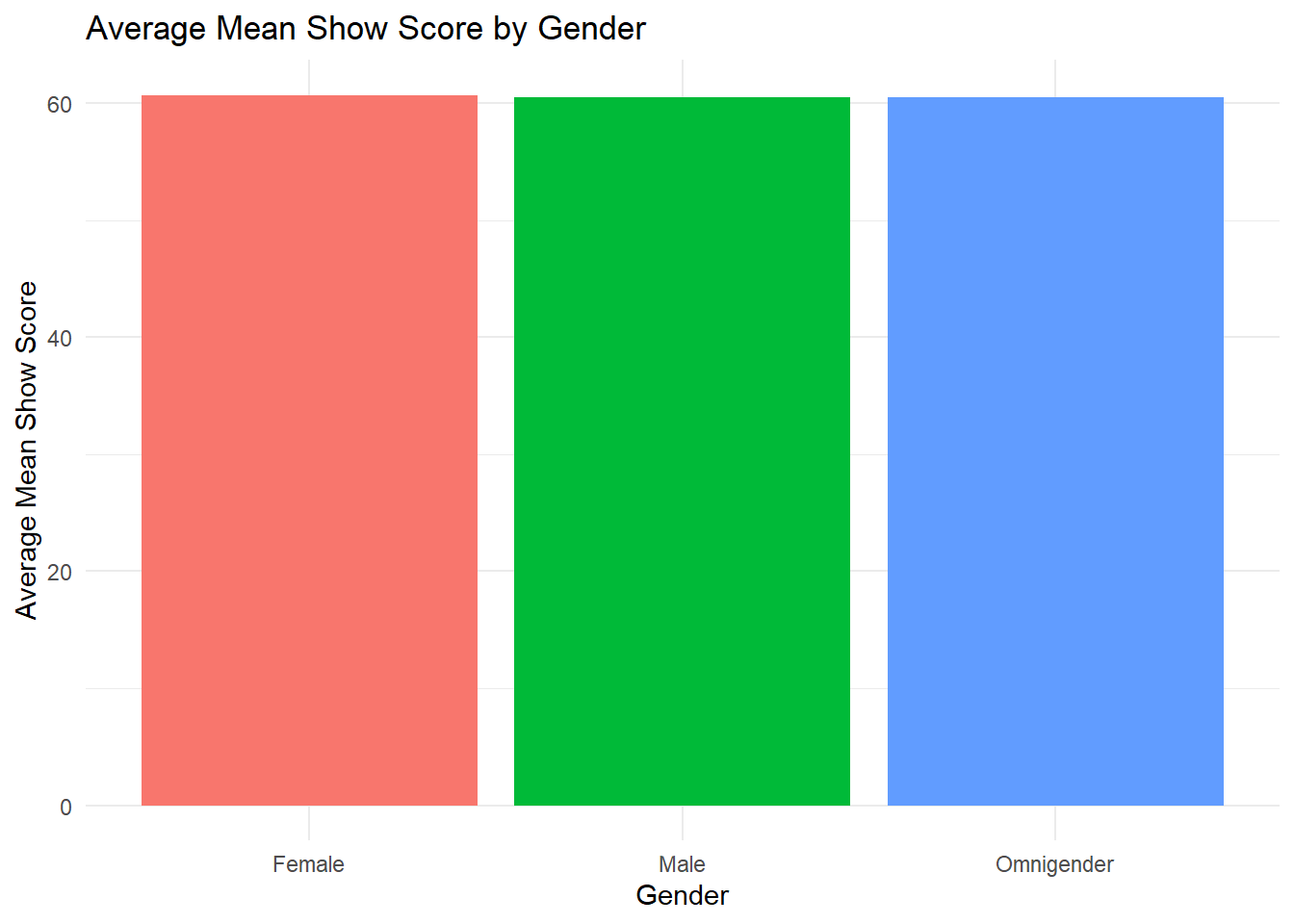

The bar chart confirms that females have a marginally higher average mean show score than males and omnigender viewers, though the difference is small. These findings suggest that overall, viewers’ show scores are relatively consistent across genders, with only minor variations.

Return to Exercise 6.2.1

Solution Quiz 6.3

Question 1:

Given the following data frames:

df1 <- data.frame(id = 1:4, name = c("Ezekiel", "Bob", "Samuel", "Diana"))

df2 <- data.frame(id = c(2, 3, 5), score = c(85, 90, 88))

Which join would return only the rows with matching id values in both data frames?

1. left_join()
   
2. right_join()
   
3. inner_join() ✓
   
4. full_join()

Question 2:

Using the same data frames, which join function retains all rows from df1 and fills unmatched rows with NA?

1. left_join() ✓
   
2. inner_join()
   
3. right_join()
   
4. full_join()

Question 3:

Which join function ensures that all rows from df2 are preserved, regardless of matches in df1?

1. left_join()
   
2. inner_join()
   
3. full_join()
   
4. right_join() ✓
   

Question 4:

What does a full join return when applied to df1 and df2?

1. Only matching rows
   
2. All rows from both data frames, with NA for unmatched entries ✓
   
3. Only rows from df1
   
4. Only rows from df2

Question 5:

In a join operation, what is the purpose of the by argument?

1. It specifies the common column(s) used to match rows between the data frames ✓
   
2. It orders the data frames
   
3. It selects which rows to retain
   
4. It converts keys to numeric values

Question 6:

If df1 contains duplicate values in the key column, what is a likely outcome of an inner join with df2?

1. The joined data frame may contain more rows than either original data frame due to duplicate matches. ✓
   
2. The join will remove all duplicates automatically.
   
3. The function will return an error.
   
4. The duplicate rows will be merged into a single row.

Question 7:

An inner join returns all rows from both data frames, regardless of whether there is a match.

1. True
   
2. False ✓
   

Question 8:

Consider the following alternative key columns:

df1 <- data.frame(studentID = 1:4, name = c("Alice", "Bob", "Charlie", "Diana"))

df2 <- data.frame(id = c(2, 3, 5), score = c(85, 90, 88))

How can you join these two data frames when the key column names differ?

1. Rename one column before joining.
   
2. Use by = c("studentID" = "id") in the join function. ✓
   
3. Use an inner join without specifying keys.
   
4. Convert the keys to factors.

Question 9:

What is a ‘foreign key’ in the context of joining datasets?

1. A column in one table that uniquely identifies each row.
   
2. A column in one table that refers to the primary key in another table. ✓
   
3. A column that has been split into multiple parts.
   
4. A column that is combined using unite().

Question 10:

Which join function would be most appropriate if you want a complete union of two datasets, preserving all rows from both?

1. full_join() ✓
   
2. inner_join()
   
3. left_join()
   
4. right_join()

Return to Quiz 6.3

Solution 6.3.1: Relational Analysis with the NYC Flights 2013 Dataset

In this solution, we explore relational data analysis using the nycflights13 dataset. We will:

1. Load and inspect the flights and planes tables.

2. Perform various join operations (inner_join, left_join, right_join, and full_join) to understand their differences.

3. Summarise the number of flights per aircraft manufacturer, handling missing data appropriately.

4. Visualise the top five manufacturers with a bar plot, displaying labels for each bar.

Setup

We install the nycflights13 package, then load it along with the tidyverse package:

# install.packages("nycflights13")

library(nycflights13)
library(tidyverse)

Inspecting the Data

We begin by inspecting the structure of the flights and planes tables to identify the available columns and the common key (tailnum).

glimpse(flights)

#> Rows: 336,776
#> Columns: 19
#> $ year           <int> 2013, 2013, 2013, 2013, 2013, 2013, 2013, 2013, 2013, 2…
#> $ month          <int> 1, 1, 1, 1, 1, 1, 1, 1, 1, 1, 1, 1, 1, 1, 1, 1, 1, 1, 1…
#> $ day            <int> 1, 1, 1, 1, 1, 1, 1, 1, 1, 1, 1, 1, 1, 1, 1, 1, 1, 1, 1…
#> $ dep_time       <int> 517, 533, 542, 544, 554, 554, 555, 557, 557, 558, 558, …
#> $ sched_dep_time <int> 515, 529, 540, 545, 600, 558, 600, 600, 600, 600, 600, …
#> $ dep_delay      <dbl> 2, 4, 2, -1, -6, -4, -5, -3, -3, -2, -2, -2, -2, -2, -1…
#> $ arr_time       <int> 830, 850, 923, 1004, 812, 740, 913, 709, 838, 753, 849,…
#> $ sched_arr_time <int> 819, 830, 850, 1022, 837, 728, 854, 723, 846, 745, 851,…
#> $ arr_delay      <dbl> 11, 20, 33, -18, -25, 12, 19, -14, -8, 8, -2, -3, 7, -1…
#> $ carrier        <chr> "UA", "UA", "AA", "B6", "DL", "UA", "B6", "EV", "B6", "…
#> $ flight         <int> 1545, 1714, 1141, 725, 461, 1696, 507, 5708, 79, 301, 4…
#> $ tailnum        <chr> "N14228", "N24211", "N619AA", "N804JB", "N668DN", "N394…
#> $ origin         <chr> "EWR", "LGA", "JFK", "JFK", "LGA", "EWR", "EWR", "LGA",…
#> $ dest           <chr> "IAH", "IAH", "MIA", "BQN", "ATL", "ORD", "FLL", "IAD",…
#> $ air_time       <dbl> 227, 227, 160, 183, 116, 150, 158, 53, 140, 138, 149, 1…
#> $ distance       <dbl> 1400, 1416, 1089, 1576, 762, 719, 1065, 229, 944, 733, …
#> $ hour           <dbl> 5, 5, 5, 5, 6, 5, 6, 6, 6, 6, 6, 6, 6, 6, 6, 5, 6, 6, 6…
#> $ minute         <dbl> 15, 29, 40, 45, 0, 58, 0, 0, 0, 0, 0, 0, 0, 0, 0, 59, 0…
#> $ time_hour      <dttm> 2013-01-01 05:00:00, 2013-01-01 05:00:00, 2013-01-01 0…

glimpse(planes)

#> Rows: 3,322
#> Columns: 9
#> $ tailnum      <chr> "N10156", "N102UW", "N103US", "N104UW", "N10575", "N105UW…
#> $ year         <int> 2004, 1998, 1999, 1999, 2002, 1999, 1999, 1999, 1999, 199…
#> $ type         <chr> "Fixed wing multi engine", "Fixed wing multi engine", "Fi…
#> $ manufacturer <chr> "EMBRAER", "AIRBUS INDUSTRIE", "AIRBUS INDUSTRIE", "AIRBU…
#> $ model        <chr> "EMB-145XR", "A320-214", "A320-214", "A320-214", "EMB-145…
#> $ engines      <int> 2, 2, 2, 2, 2, 2, 2, 2, 2, 2, 2, 2, 2, 2, 2, 2, 2, 2, 2, …
#> $ seats        <int> 55, 182, 182, 182, 55, 182, 182, 182, 182, 182, 55, 55, 5…
#> $ speed        <int> NA, NA, NA, NA, NA, NA, NA, NA, NA, NA, NA, NA, NA, NA, N…
#> $ engine       <chr> "Turbo-fan", "Turbo-fan", "Turbo-fan", "Turbo-fan", "Turb…

The flights table contains 336,776 rows and 19 columns, whereas the planes table contains 3,322 rows and 9 columns. Both tables share the tailnum field, which we will use to link them.

Relational Analysis with Joins

1. Inner Join

An inner join returns only those rows that have matching keys in both tables. In this case, only flights with a corresponding plane record are included.

inner_join_result <- inner_join(flights, planes, by = "tailnum")

inner_join_result

#> # A tibble: 284,170 × 27
#>    year.x month   day dep_time sched_dep_time dep_delay arr_time sched_arr_time
#>     <int> <int> <int>    <int>          <int>     <dbl>    <int>          <int>
#>  1   2013     1     1      517            515         2      830            819
#>  2   2013     1     1      533            529         4      850            830
#>  3   2013     1     1      542            540         2      923            850
#>  4   2013     1     1      544            545        -1     1004           1022
#>  5   2013     1     1      554            600        -6      812            837
#>  6   2013     1     1      554            558        -4      740            728
#>  7   2013     1     1      555            600        -5      913            854
#>  8   2013     1     1      557            600        -3      709            723
#>  9   2013     1     1      557            600        -3      838            846
#> 10   2013     1     1      558            600        -2      849            851
#> # ℹ 284,160 more rows
#> # ℹ 19 more variables: arr_delay <dbl>, carrier <chr>, flight <int>,
#> #   tailnum <chr>, origin <chr>, dest <chr>, air_time <dbl>, distance <dbl>,
#> #   hour <dbl>, minute <dbl>, time_hour <dttm>, year.y <int>, type <chr>,
#> #   manufacturer <chr>, model <chr>, engines <int>, seats <int>, speed <int>,
#> #   engine <chr>

Since flights has 336,776 rows, the inner join result of 284,170 rows indicates that some flights lack a matching tailnum in the planes table (or have missing tailnum values).

2. Left Join {.unnumbered}

A left join returns all rows from the left table (flights) and any matching rows from the right table (planes). Unmatched plane columns are filled with NA.

left_join_result <- left_join(flights, planes, by = "tailnum")

left_join_result

#> # A tibble: 336,776 × 27
#>    year.x month   day dep_time sched_dep_time dep_delay arr_time sched_arr_time
#>     <int> <int> <int>    <int>          <int>     <dbl>    <int>          <int>
#>  1   2013     1     1      517            515         2      830            819
#>  2   2013     1     1      533            529         4      850            830
#>  3   2013     1     1      542            540         2      923            850
#>  4   2013     1     1      544            545        -1     1004           1022
#>  5   2013     1     1      554            600        -6      812            837
#>  6   2013     1     1      554            558        -4      740            728
#>  7   2013     1     1      555            600        -5      913            854
#>  8   2013     1     1      557            600        -3      709            723
#>  9   2013     1     1      557            600        -3      838            846
#> 10   2013     1     1      558            600        -2      753            745
#> # ℹ 336,766 more rows
#> # ℹ 19 more variables: arr_delay <dbl>, carrier <chr>, flight <int>,
#> #   tailnum <chr>, origin <chr>, dest <chr>, air_time <dbl>, distance <dbl>,
#> #   hour <dbl>, minute <dbl>, time_hour <dttm>, year.y <int>, type <chr>,
#> #   manufacturer <chr>, model <chr>, engines <int>, seats <int>, speed <int>,
#> #   engine <chr>

The result retains all 336,776 flights. Where there is no matching plane information, the plane-related fields will be NA.

3. Right Join {.unnumbered}

A right join returns all rows from the right table (planes) and any matching rows from the left table (flights). This join emphasises the planes, potentially including planes that did not appear in any flight record.

right_join_result <- right_join(flights, planes, by = "tailnum")

right_join_result

#> # A tibble: 284,170 × 27
#>    year.x month   day dep_time sched_dep_time dep_delay arr_time sched_arr_time
#>     <int> <int> <int>    <int>          <int>     <dbl>    <int>          <int>
#>  1   2013     1     1      517            515         2      830            819
#>  2   2013     1     1      533            529         4      850            830
#>  3   2013     1     1      542            540         2      923            850
#>  4   2013     1     1      544            545        -1     1004           1022
#>  5   2013     1     1      554            600        -6      812            837
#>  6   2013     1     1      554            558        -4      740            728
#>  7   2013     1     1      555            600        -5      913            854
#>  8   2013     1     1      557            600        -3      709            723
#>  9   2013     1     1      557            600        -3      838            846
#> 10   2013     1     1      558            600        -2      849            851
#> # ℹ 284,160 more rows
#> # ℹ 19 more variables: arr_delay <dbl>, carrier <chr>, flight <int>,
#> #   tailnum <chr>, origin <chr>, dest <chr>, air_time <dbl>, distance <dbl>,
#> #   hour <dbl>, minute <dbl>, time_hour <dttm>, year.y <int>, type <chr>,
#> #   manufacturer <chr>, model <chr>, engines <int>, seats <int>, speed <int>,
#> #   engine <chr>

Because there are fewer planes than flights, and most flights have matching planes, the result (284,170 rows) is similar to the inner join count. Planes never used in any flight appear with NA for flight-specific columns.

4. Full Join {.unnumbered}

A full join includes all rows from both tables, matching where possible. Any rows that do not match in either table are shown with NA in the missing fields.

full_join_result <- full_join(flights, planes, by = "tailnum")

full_join_result

#> # A tibble: 336,776 × 27
#>    year.x month   day dep_time sched_dep_time dep_delay arr_time sched_arr_time
#>     <int> <int> <int>    <int>          <int>     <dbl>    <int>          <int>
#>  1   2013     1     1      517            515         2      830            819
#>  2   2013     1     1      533            529         4      850            830
#>  3   2013     1     1      542            540         2      923            850
#>  4   2013     1     1      544            545        -1     1004           1022
#>  5   2013     1     1      554            600        -6      812            837
#>  6   2013     1     1      554            558        -4      740            728
#>  7   2013     1     1      555            600        -5      913            854
#>  8   2013     1     1      557            600        -3      709            723
#>  9   2013     1     1      557            600        -3      838            846
#> 10   2013     1     1      558            600        -2      753            745
#> # ℹ 336,766 more rows
#> # ℹ 19 more variables: arr_delay <dbl>, carrier <chr>, flight <int>,
#> #   tailnum <chr>, origin <chr>, dest <chr>, air_time <dbl>, distance <dbl>,
#> #   hour <dbl>, minute <dbl>, time_hour <dttm>, year.y <int>, type <chr>,
#> #   manufacturer <chr>, model <chr>, engines <int>, seats <int>, speed <int>,
#> #   engine <chr>

Here, we see 336,776 rows again. Since flights is larger, the full join remains at 336,776. Additional planes that are not used in any flights appear with NA in flight-related columns but do not increase the total row count.

Summary Table: Flights per Aircraft Manufacturer

Next, we create a summary table of flights per aircraft manufacturer. We use the left join result (left_join_result) so that all flights remain, even if plane information is missing. We label these missing values as "Unknown".

manufacturer_summary <- left_join_result %>%
  mutate(manufacturer = if_else(is.na(manufacturer), "Unknown", manufacturer)) %>%
  count(manufacturer, sort = TRUE)

manufacturer_summary

#> # A tibble: 36 × 2
#>    manufacturer                      n
#>    <chr>                         <int>
#>  1 BOEING                        82912
#>  2 EMBRAER                       66068
#>  3 Unknown                       52606
#>  4 AIRBUS                        47302
#>  5 AIRBUS INDUSTRIE              40891
#>  6 BOMBARDIER INC                28272
#>  7 MCDONNELL DOUGLAS AIRCRAFT CO  8932
#>  8 MCDONNELL DOUGLAS              3998
#>  9 CANADAIR                       1594
#> 10 MCDONNELL DOUGLAS CORPORATION  1259
#> # ℹ 26 more rows

From the output, BOEING has the highest number of flights (82,912), followed by EMBRAER (66,068). A substantial number of flights (52,606) have no matching manufacturer data, labelled as Unknown.

Bar Plot: Top Five Aircraft Manufacturers

Finally, we select the top five manufacturers and visualise them with a bar plot, displaying the exact flight count above each bar.

top_manufacturers <- manufacturer_summary %>%
  slice_max(n, n = 5)

top_manufacturers |> ggplot(aes(x = reorder(manufacturer, -n), y = n, fill = manufacturer)) +
  geom_col(show.legend = FALSE, width = 0.4) +
  # Display the exact value above each bar, with thousand separators
  geom_text(aes(label = scales::comma(n)), vjust = -0.3) +
  # Apply thousand separators to the y-axis
  scale_y_continuous(labels = scales::comma) +
  labs(
    x = "Manufacturer",
    y = "Number of Flights",
    title = "Top 5 Aircraft Manufacturers by Number of Flights"
  ) +
  theme_minimal()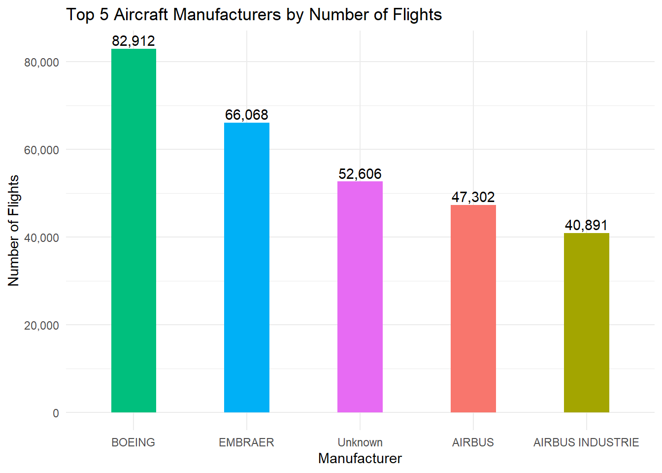

This chart confirms that Boeing-manufactured planes account for the largest share of flights, followed by Embraer. The “Unknown” category represents flights for which plane data is missing in the planes table. You will learn more about data visualisation techniques in Chapter 7 of this book.

Return to Exercise 6.3.1

Lab 7: Data Visualisation

Solution Quiz 7.1

Question 1:

Which principle is the foundation of ggplot2’s structured approach to building graphs?

1. The Aesthetic Mapping Principle
   
2. The Facet Wrapping Technique
   
3. The Grammar of Graphics ✓
   
4. The Scaling Transformation Theory

Question 2:

In a ggplot2 plot, which of the following best describes the role of aes()?

1. It specifies the dataset to be plotted.
   
2. It defines statistical transformations to apply to the data.
   
3. It maps data variables to visual properties, like colour or size. ✓
   
4. It sets the coordinate system for the plot.

Question 3:

If you want to display the distribution of a single continuous variable and identify its modality and skewness, which geom is most appropriate?

1. geom_point()
   
2. geom_bar()
   
3. geom_histogram() ✓
   
4. geom_col()

Question 4:

When creating a boxplot to show the variation of a continuous variable across multiple categories, what do the “whiskers” typically represent?

1. The median value and the mean value.
   
2. The full range of the data, excluding outliers.
   
3. One standard deviation above and below the mean.
   
4. The maximum and minimum values after applying a 1.5 * IQR rule. ✓

Question 5:

You have a dataset with a categorical variable Region and a continuous variable Sales. You want to compare total sales across different regions. Which geom and aesthetic mapping would be most appropriate?

1. geom_bar(aes(x = Region)), which internally counts the occurrences of each region.

2. geom_col(aes(x = Region, y = Sales)), which uses the actual Sales values for the bar heights. ✓
   

3. geom_line(aes(x = Region, y = Sales)), connecting points across regions.

4. geom_area(aes(x = Region, y = Sales)), to show cumulative totals over regions.

Question 6:

If you want to add a smoothing line (e.g., a regression line) to a scatter plot created with geom_point(), which geom should you use and with what parameter to fit a linear model without confidence intervals?

1. geom_smooth(method = "lm", se = FALSE) ✓
   

2. geom_line(stat = "lm", se = TRUE)

3. geom_line(method = "regress", se = FALSE)

4. geom_smooth(method = "reg", confint = FALSE)

Question 7:

Consider you have a factor variable cyl representing the number of cylinders in the mtcars dataset. If you want to create multiple plots (small multiples) for each value of cyl, which ggplot2 function can you use?

1. facet_wrap(~ cyl) ✓
   

2. facet_side(~ cyl)

3. group_by(cyl) followed by multiple geom_point() calls

4. geom_facet(cyl)

Question 8:

Which of the following statements about ggsave() is true?

1. ggsave() must be called before creating any plots for it to work correctly.

2. ggsave() saves the last plot displayed, and you can control the output format by specifying the file extension. ✓
   

3. ggsave() cannot control the width, height, or resolution of the output image.

4. ggsave() only saves plots as PDF files.

Question 9:

What is the purpose of setting group aesthetics in a ggplot, for example in a line plot?

1. To change the colour scale of all elements.
   
2. To ensure that discrete categories are grouped together for transformations like smoothing.
   
3. To define which points belong to the same series, enabling lines to connect points within groups instead of mixing data across categories. ✓
   
4. To modify only the legend titles and labels.

Question 10:

When customizing themes, which of the following options is NOT directly controlled by a theme() function in ggplot2?

1. Axis text size, angle, and colour.
   
2. Background grid lines and panel background.
   
3. The raw data values in the dataset. ✓
   
4. The plot title alignment and style.

Return to Quiz 7.1

Solution Quiz 7.2

Question 1:

Which of the following is a key advantage of using Base R graphics for exploratory data analysis?

1. They require additional packages.
   
2. They offer a quick, function-based approach with no dependencies ✓
   
3. They utilise a layered grammar for complex plotting.
   
4. They automatically produce interactive visualisations.

Question 2:

Which function is the generic function in Base R for creating scatterplots, line graphs, and other basic plots?

1. hist()
   
2. plot() ✓
   
3. boxplot()
   
4. barplot()

Question 3:

Which function in Base R is specifically used to display data distributions as histograms?

1. pie()
   
2. plot()
   
3. hist() ✓
   
4. boxplot()

Question 4:

What is the purpose of the breaks argument in the hist() function?

1. To set the colour of the bars.
   
2. To determine the bin width for the histogram ✓
   
3. To label the axes.
   
4. To specify the main title.

Question 5:

Which graphical parameter in Base R is used to specify the colour of plot elements?

1. pch
   
2. lty
   
3. col ✓
   
4. cex

Question 6:

The pch parameter in Base R plots is used to control:

1. The type of point symbol displayed ✓
   
2. The line thickness.
   
3. The overall scaling of plot elements.
   
4. The arrangement of multiple plots.

Question 7:

Which function in Base R is used to adjust global graphical settings, such as margins and layout arrangements?

1. plot()
   
2. par() ✓
   
3. hist()
   
4. boxplot()

Question 8:

In a Base R scatter plot, which function is used to add a regression line?

1. lines()
   
2. abline() ✓
   
3. curve()
   
4. segments()

Question 9:

What is one of the main reasons Base R graphics are considered advantageous over ggplot2 for certain tasks?

1. They require no additional packages since they are built into R ✓
   
2. They offer more extensive theme options.
   
3. They are better suited for interactive visualisations.
   
4. They automatically manage data transformations.

Question 10:

When saving a Base R plot using the png() function, what is the purpose of calling dev.off() afterwards?

1. To display the saved plot.
   
2. To open the saved file in a new window.
   
3. To close the graphics device and finalise the output file ✓
   
4. To reset all graphical parameters.

Return to Quiz 7.2

Solution 7.1.2: Reproducing the Smoking, Gender, and Lifespan Chart

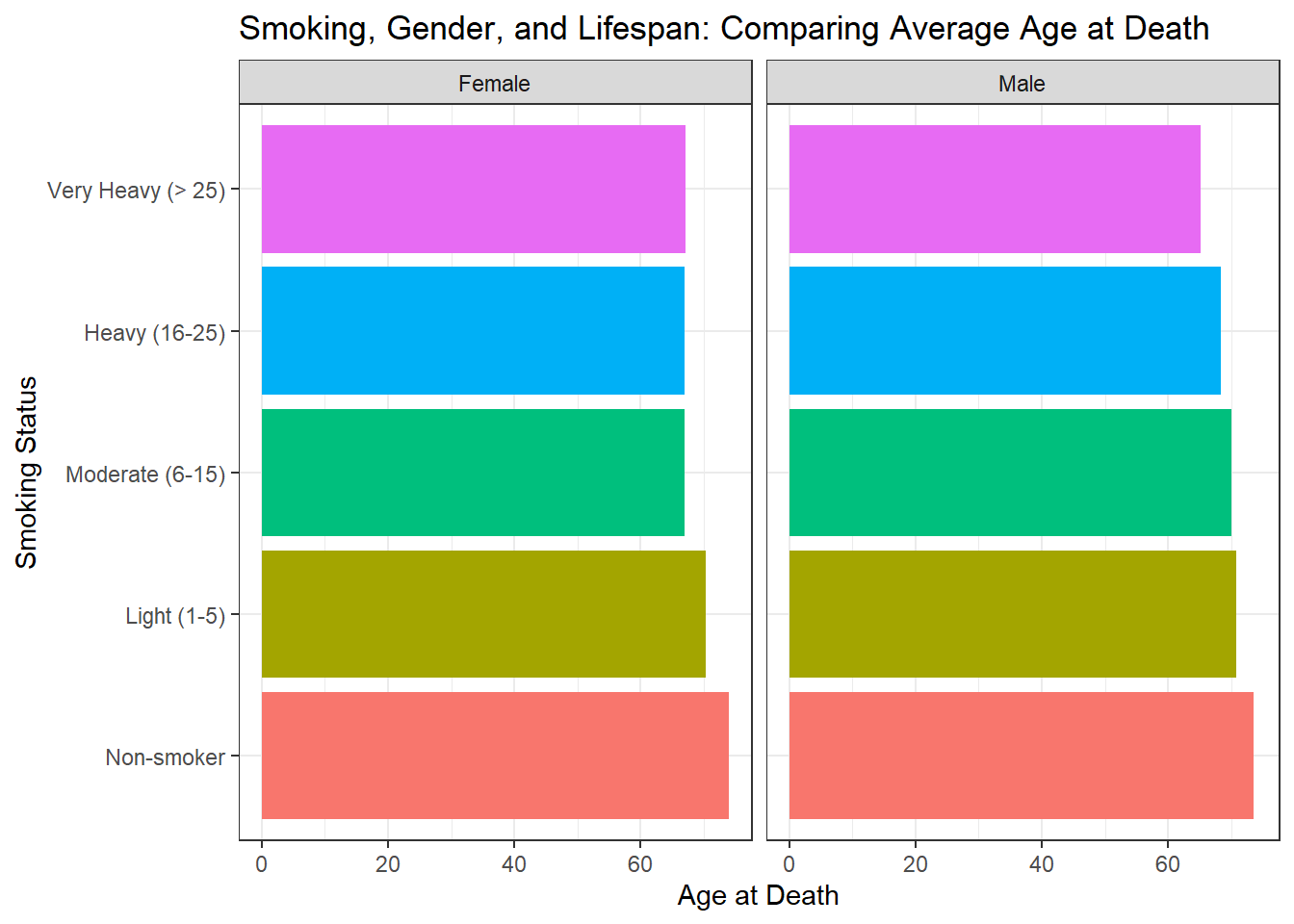
In this solution, we will demonstrate how to reproduce the chart that compares the average age at death by smoking status for both males and females. The data comes from the Framingham Heart Study and is contained in the heart dataset. Our aim is to filter, summarise, and visualise the data using dplyr and ggplot2.

Importing and Inspecting the Data

First, we import the heart.xlsx file from the r-data directory using read_excel() and inspect its structure with functions such as glimpse(). This step ensures that the dataset has been loaded correctly and familiarises us with its variables.

library(tidyverse)
library(readxl)
library(janitor)

# Import the dataset from the r-data directory
heart <- read_excel("r-data/heart.xlsx")
heart <- heart |> clean_names()

# Inspect the data structure
glimpse(heart)

#> Rows: 5,209
#> Columns: 17
#> $ status         <chr> "Dead", "Dead", "Alive", "Alive", "Alive", "Alive", "Al…
#> $ death_cause    <chr> "Other", "Cancer", NA, NA, NA, NA, NA, "Other", NA, "Ce…
#> $ age_ch_ddiag   <dbl> NA, NA, NA, NA, NA, NA, NA, NA, NA, NA, NA, 57, 55, 79,…
#> $ sex            <chr> "Female", "Female", "Female", "Female", "Male", "Female…
#> $ age_at_start   <dbl> 29, 41, 57, 39, 42, 58, 36, 53, 35, 52, 39, 33, 33, 57,…
#> $ height         <dbl> 62.50, 59.75, 62.25, 65.75, 66.00, 61.75, 64.75, 65.50,…
#> $ weight         <dbl> 140, 194, 132, 158, 156, 131, 136, 130, 194, 129, 179, …
#> $ diastolic      <dbl> 78, 92, 90, 80, 76, 92, 80, 80, 68, 78, 76, 68, 90, 76,…
#> $ systolic       <dbl> 124, 144, 170, 128, 110, 176, 112, 114, 132, 124, 128, …
#> $ mrw            <dbl> 121, 183, 114, 123, 116, 117, 110, 99, 124, 106, 133, 1…
#> $ smoking        <dbl> 0, 0, 10, 0, 20, 0, 15, 0, 0, 5, 30, 0, 0, 15, 30, 10, …
#> $ age_at_death   <dbl> 55, 57, NA, NA, NA, NA, NA, 77, NA, 82, NA, NA, NA, NA,…
#> $ cholesterol    <dbl> NA, 181, 250, 242, 281, 196, 196, 276, 211, 284, 225, 2…
#> $ chol_status    <chr> NA, "Desirable", "High", "High", "High", "Desirable", "…
#> $ bp_status      <chr> "Normal", "High", "High", "Normal", "Optimal", "High", …
#> $ weight_status  <chr> "Overweight", "Overweight", "Overweight", "Overweight",…
#> $ smoking_status <chr> "Non-smoker", "Non-smoker", "Moderate (6-15)", "Non-smo…

The heart dataset comprises 5,209 observations and 17 variables, including important fields such as sex, age_at_death, and smoking_status.

We then transform the variable smoking_status as ordered factor:

heart <- heart |>
  mutate(smoking_status = factor(smoking_status,
    levels = c(
      "Non-smoker", "Light (1-5)", "Moderate (6-15)", "Heavy (16-25)",
      "Very Heavy (> 25)"
    )
  ))

Filtering and Summarising the Data

Next, we filter the data to remove any observations with missing values in the smoking_status column. We then group the data by both smoking_status and sex, calculating the mean of age_at_death for each group. This produces a new dataset containing the average age at death per smoking category and gender.

heart_summary <- heart %>%
  filter(!is.na(smoking_status)) %>%
  group_by(smoking_status, sex) %>%
  summarise(
    avg_age_at_death = mean(age_at_death, na.rm = TRUE),
    .groups = "drop"
  )

# Display the summarised data
heart_summary

#> # A tibble: 10 × 3
#>    smoking_status    sex    avg_age_at_death
#>    <fct>             <chr>             <dbl>
#>  1 Non-smoker        Female             73.9
#>  2 Non-smoker        Male               73.5
#>  3 Light (1-5)       Female             70.4
#>  4 Light (1-5)       Male               70.7
#>  5 Moderate (6-15)   Female             67.1
#>  6 Moderate (6-15)   Male               70.1
#>  7 Heavy (16-25)     Female             67.0
#>  8 Heavy (16-25)     Male               68.3
#>  9 Very Heavy (> 25) Female             67.2
#> 10 Very Heavy (> 25) Male               65.1

Visualising the Results

We then use ggplot2 to create a horizontal bar chart. In this visualisation, the x-axis displays the average age at death, while the y-axis represents the different smoking status categories. The chart is facetted by sex to provide separate panels for females and males. The fill colour differentiates the smoking categories, and the plot includes a clear title and axis labels.

heart_summary |>
  ggplot(aes(x = avg_age_at_death, y = smoking_status, fill = smoking_status)) +
  geom_col(show.legend = FALSE) +
  facet_wrap(~sex) +
  labs(
    title = "Smoking, Gender, and Lifespan: Comparing Average Age at Death",
    x = "Age at Death",
    y = "Smoking Status"
  ) +
  theme_bw()

Interpretation

This chart clearly illustrates how the average age at death differs across smoking categories and between genders. Typically, non-smokers appear to have a higher average age at death compared to heavier smokers. Additionally, subtle differences between females and males can be observed, highlighting the significance of considering both smoking status and sex when analysing lifespan.

Return to Exercise 7.1.2

Lab 8: Statistical Concept

Solution Quiz 8.0

Question 1:

Data that focuses on characteristics or qualities rather than numbers is known as:

1. Quantitative data
   
2. Discrete data
   
3. Qualitative data ✓
   
4. Continuous data

Question 2:

Which of the following is an example of discrete data?

1. The height of students in a class
   
2. The number of cars in a parking lot ✓
   
3. The amount of rainfall in a day
   
4. The time taken to complete a task

Question 3:

Quantitative data that can take on any value within a given range is referred to as:

1. Categorical data
   
2. Nominal data
   
3. Discrete data
   
4. Continuous data ✓
   

Question 4:

Qualitative data differs from quantitative data because qualitative data:
a) Can only be expressed with numbers
b) Has meaningful mathematical operations
c) Describes categories or groups ✓  d) Is always collected from secondary sources

Question 5:

Primary data refers to data that:

1. Has been previously published by others
   
2. Comes directly from observation or experiment ✓
   
3. Is always collected online
   
4. Is obtained only from government agencies

Question 6:

A list of colours observed in a garden (e.g., red, yellow, green) is an example of:

1. Quantitative continuous data
   
2. Quantitative discrete data
   
3. Qualitative data ✓
   
4. Secondary data

Question 7:

Which of the following statements is true?

1. Data is always meaningful without analysis
   
2. Data, once processed, is known as information ✓
   
3. Data and information are identical concepts
   
4. Information is just another term for data collection

Question 8:

A measurement like “23 people attended the seminar” is an example of:

1. Qualitative data
   
2. Continuous data
   
3. Discrete data ✓
   
4. Nominal scale data

Question 9:

Data collected for the first time for a specific research purpose is known as:

1. Secondary data
   
2. Primary data ✓
   
3. Nominal data
   
4. Discrete data

Question 10:

A researcher using census data from a national statistics bureau is working with:

1. Primary data
   
2. Secondary data ✓
   
3. Continuous data
   
4. Nominal data

Return to Quiz 8.0

Solution Quiz 8.1

Question 1:

A complete set of elements (people, items) that we are interested in studying is called a:

1. Sample
   
2. Population ✓
   
3. Parameter
   
4. Statistic

Question 2:

A subset of a population used to make inferences about the population is called a:

1. Population
   
2. Sample ✓
   
3. Statistic
   
4. Parameter

Question 3:

A value that describes a characteristic of an entire population (e.g., population mean) is known as a:

1. Statistic
   
2. Parameter ✓
   
3. Variable
   
4. Sample estimate

Question 4:

A value computed from sample data (e.g., sample mean) that is used to estimate a population parameter is called a:

1. Parameter
   
2. Statistic ✓
   
3. Variable
   
4. Census

Question 5:

Why do we often rely on samples rather than studying entire populations?

1. It is always more accurate.
   
2. Populations do not have parameters.
   
3. Sampling is often more feasible, less costly, and time-efficient ✓
   
4. Populations are always small and uninteresting.

Question 6:

Statistical thinking involves understanding how to:

1. Manipulate data without purpose
   
2. Draw meaningful conclusions from data under uncertainty ✓
   
3. Avoid using data in decision-making
   
4. Ignore variability in data

Question 7:

If a population parameter is \(\mu\), the corresponding sample statistic used to estimate it is typically:

1. s
   
2. \(\sigma\)
   
3. \(\bar{x}\) ✓
   
4. p

Question 8:

When we attempt to understand the variability in data and the uncertainty in our conclusions, we are engaging in:

1. Statistical thinking ✓
   
2. Non-statistical reasoning
   
3. Data neglect
   
4. Parameter ignorance

Question 9:

If it’s too expensive or impractical to study an entire population, we often conduct a:

1. Census
   
2. Biased survey
   
3. Sample study ✓
   
4. Parameter test

Question 10:

The process of using sample data to make conclusions about a larger population is known as:

1. Data summarisation
   
2. Descriptive statistics
   
3. Statistical inference ✓
   
4. Variable classification

Return to Quiz 8.1

Solution- Exercise 8.1.2: Professor Francisca - A Generous Giver

Professor Francisca, the Vice-Chancellor of Thomas Adewumi University, Kwara, Nigeria, and a Professor of Computer Science, is known for her generosity. Each week, she awards monetary prizes (in dollars) to the best student in the weekly Computer Science assignment for the DTS 204 module. The prize amounts are as follows:

495, 503, 503, 498, 503, 505, 503, 500, 501, 489, 498, 488, 499, 497, 508, 507, 507, 509, 508, 503.

Using R, complete the following tasks to analyze the data:

Task 1: Central Tendency

1. Calculate the Mean

   money <- c(495, 503, 503, 498, 503, 505, 503, 500, 501, 489, 498, 488, 499, 497, 508, 507, 507, 509, 508, 503)
   mean(money)

   #> [1] 501.2

2. Calculate the Median

   median(money)

   #> [1] 503

3. Determine the Mode

   statistical_mode <- function(x) {
     uniqx <- unique(x)
     uniqx[which.max(tabulate(match(x, uniqx)))]
   }
   statistical_mode(money)

   #> [1] 503

Task 2: Measure of Spread

1. Calculate the Range

   range_value <- max(money) - min(money)
   range_value

   #> [1] 21

2. Determine the Standard Deviation

   sd(money)

   #> [1] 5.881282

   The standard deviation helps us understand the consistency of the amounts given out.

3. Find the Variance

   var(money)

   #> [1] 34.58947

   Variance is the square of the standard deviation.

Task 3: Measure of Partition

1. Calculate the Interquartile Range (IQR)

   IQR(money)

   #> [1] 7.5

   The IQR measures the spread of the middle 50% of the amounts.

2. Find the Quartiles

   quantile(money)

   #>    0%   25%   50%   75%  100% 
   #> 488.0 498.0 503.0 505.5 509.0

   The quartiles reveal the distribution of the amounts.

3. Calculate Percentile Ranks

   To determine the percentile ranks for $488 (minimum), $509 (maximum), and $503:

   ecdf_money <- ecdf(money)
   percentile_488 <- ecdf_money(488) * 100 # Percentile rank of $488
   
   percentile_509 <- ecdf_money(509) * 100 # Percentile rank of $509
   
   percentile_503 <- ecdf_money(503) * 100 # Percentile rank of $503

   • Percentile rank of $488: Indicates the percentage of amounts less than or equal to $488.

   • Percentile rank of $509: Indicates the percentage of amounts less than or equal to $509.

   • Percentile rank of $503: Indicates the position of $503 within the distribution.

Interpretation

• The mean amount is $501.2, while the median is $503. This slight difference suggests a relatively symmetrical distribution with a slight skew.

• The mode is $503, indicating that this amount was given out most frequently.

• The range of $21 shows the variability between the smallest and largest amounts.

• The standard deviation and variance quantify the overall spread of the amounts.

• The IQR compares the variability of the middle 50% to the overall range, revealing insights about data dispersion.

• The quartiles help understand how the amounts are distributed across the dataset.

• The percentile ranks position specific amounts within the overall distribution, providing context for their relative standing.

Return to Exercise 8.1.2

Solution Quiz 8.2

Question 1:

Which set of values is included in a five-number summary?

1. Mean, Median, Mode, IQR, Standard Deviation
   
2. Minimum, Q1, Median, Q3, Maximum ✓
   
3. Minimum, Mean, Mode, Maximum, Range
   
4. Q1, Q2, Q3, Q4, Q5

Question 2:

The interquartile range (IQR) is calculated as:

1. Q2 - Q1
   
2. Q3 - Median
   
3. Q3 - Q1 ✓
   
4. Median - Minimum

Question 3:

A boxplot is useful for:

1. Displaying frequencies of categorical data
   
2. Showing the distribution and identifying outliers ✓
   
3. Calculating correlations between variables
   
4. Displaying only the mean value

Question 4:

Which value in a five-number summary represents the median of the entire dataset?

1. Q1
   
2. Q2 (Median) ✓
   
3. Q3
   
4. Minimum

Question 5:

If a dataset has many outliers, a boxplot can help by:

1. Ignoring them completely
   
2. Highlighting them as points beyond the whiskers ✓
   
3. Removing them automatically
   
4. Converting them to the mean value

Question 6:

The IQR focuses on the middle 50% of data, making it a good measure of:

1. Central tendency
   
2. Spread that is not influenced by extreme values ✓
   
3. Correlation
   
4. Nominal categories

Question 7:

In R, the boxplot() function by default displays:

1. A histogram
   
2. A correlation matrix
   
3. A five-number summary depiction ✓
   
4. A scatter plot

Question 8:

The difference between the maximum and minimum values in a dataset is called the:

1. Standard deviation
   
2. IQR
   
3. Range ✓
   
4. Variance

Question 9:

A box-and-whisker plot typically does NOT show:

1. Median
   
2. Outliers
   
3. Mean ✓
   
4. Interquartile range

Question 10:

When comparing two datasets using boxplots placed side by side, you can quickly assess differences in:

1. Central tendency and spread ✓
   
2. Exact individual data points
   
3. Correlation coefficients
   
4. Detailed frequency distributions

Return to Quiz 8.2

Solution- Exercise 8.2.1

Thirty farmers were surveyed about the number of farm workers they employ during a typical harvest season in Igboho, Oyo State, Nigeria. Their responses are as follows:

4, 5, 6, 5, 1, 2, 8, 0, 4, 6, 7, 8, 4, 6, 7, 9, 8, 6, 7, 5, 5, 4, 2, 1, 9, 3, 3, 4, 6, 4.

Task 1: Calculate the Mean, Median, and Mode

Calculating the Mean:

The mean is the sum of all observations divided by the number of observations.

Total number of farm workers employed:

\[\text{Total} = 4 + 5 + 6 + \cdots + 4 = 149\]

Number of observations (n): \(30\)

\[\text{Mean} = \frac{\text{Total}}{n} = \frac{149}{30} \approx 4.97\]

Calculating the Median:

The median is the middle value when the data are arranged in ascending order.

First, arrange the data:

0, 1, 1, 2, 2, 3, 3, 4, 4, 4, 4, 4, 5, 5, 5, 5, 6, 6, 6, 6, 6, 7, 7, 7, 7, 8, 8, 8, 9, 9

Since there are 30 observations (an even number), the median is the average of the 15th and 16th values.

15th value: 5

16th value: 5

Median:

\[ \text{Median} = \frac{5 + 5}{2} = 5 \]

Calculating the Mode:

The mode is the value that occurs most frequently.

Frequency of each number:

• 4 occurs 5 times
• 6 occurs 5 times

Both 4 and 6 have the highest frequency.

Therefore, the dataset is bimodal with modes at 4 and 6.

This is how to calculate the mean, median, and mode in R:

farm_workers <- c(4, 5, 6, 5, 1, 2, 8, 0, 4, 6, 7, 8, 4, 6, 7, 9, 8, 6, 7, 5, 5, 4, 2, 1, 9, 3, 3, 4, 6, 4)

# Mean
mean(farm_workers)

#> [1] 4.966667

# Median
median(farm_workers)

#> [1] 5

# Mode
statistical_mode <- function(x) {
  uniqx <- unique(x)
  freq <- tabulate(match(x, uniqx))
  uniqx[freq == max(freq)]
}

statistical_mode(farm_workers)

#> [1] 4

Task 2: Determine the Range and Standard Deviation

Calculating the Range:

The range is the difference between the maximum and minimum values.

Minimum value:

\[ \text{Min} = 0 \]

Maximum value:

\[ \text{Max} = 9 \]

Range:

\[ \text{Range} = \text{Max} - \text{Min} = 9 - 0 = 9 \]

Calculating the Standard Deviation:

The standard deviation measures the amount of variation or dispersion in the dataset.

This is how to calculate the range and standard deviation in R:

# Range
range_values <- range(farm_workers)
range_values # Outputs the minimum and maximum values

#> [1] 0 9

range <- diff(range_values)
range # Outputs the range

#> [1] 9

# Standard Deviation
sd(farm_workers)

#> [1] 2.385059

Task 3: Create a Box-and-Whisker Plot of the Distribution

To visualise the distribution of the number of farm workers employed, you can create a box-and-whisker plot.

This is how to create the box plot in R:

boxplot(farm_workers,
  main = "Box-and-Whisker Plot of Number of Farm Workers",
  ylab = "Number of Workers",
  col = "green"
)

Return to Exercise 8.2.1

Solution Quiz 8.3

Question 1:

A scale that categorises data without any order is known as:

1. Nominal ✓
   
2. Ordinal
   
3. Interval
   
4. Ratio

Question 2:

Which scale provides both order and equal intervals but no true zero point?

1. Nominal
   
2. Ordinal
   
3. Interval ✓
   
4. Ratio

Question 3:

Which scale allows for meaningful ratios and has a true zero?

1. Nominal
   
2. Ordinal
   
3. Interval
   
4. Ratio ✓
   

Question 4:

Educational levels ranked as “Primary, Secondary, Tertiary” represent which scale?

1. Nominal
   
2. Ordinal ✓
   
3. Interval
   
4. Ratio

Question 5:

Temperatures in Celsius or Fahrenheit are examples of which scale?

1. Nominal
   
2. Ordinal
   
3. Interval ✓
   
4. Ratio

Question 6:

Blood types (A, B, AB, O) are measured on which scale?

1. Nominal ✓
   
2. Ordinal
   
3. Interval
   
4. Ratio

Question 7:

The number of items sold in a store (e.g., 0, 5, 10 units) is best described by which scale?

1. Nominal
   
2. Ordinal
   
3. Ratio ✓
   
4. Interval

Question 8:

Customer satisfaction ratings (e.g., Satisfied, Neutral, Unsatisfied) belong to which scale?

1. Nominal
   
2. Ordinal ✓
   
3. Interval
   
4. Ratio

Question 9:

A key difference between interval and ratio scales is that ratio scales have:

1. Categories only
   
2. A meaningful zero point ✓
   
3. No ordering capability
   
4. Equal intervals that are meaningless

Question 10:

IQ scores are often treated as which type of scale?

1. Nominal
   
2. Ordinal
   
3. Interval ✓
   
4. Ratio

Return to Quiz 8.3

Solution-Exercise 8.3.1: Identify the Scale

1. Blood pressure readings (e.g., 120 mmHg, 130 mmHg)

   Answer: Interval Scale

   Explanation:

   • Numerical Data with Equal Intervals: Blood pressure readings are numerical values where the difference between measurements is consistent (e.g., the difference between 120 mmHg and 130 mmHg is the same as between 130 mmHg and 140 mmHg).

   • No True Zero Point: In the context of blood pressure, a reading of 0 mmHg is not meaningful for living humans; it does not represent the absence of blood pressure but rather an unmeasurable or non-viable state.

   • Implications: Because there is no absolute zero, ratios are not meaningful (e.g., we cannot say that 120 mmHg is twice as much as 60 mmHg in a meaningful way).

2. Type of car owned (e.g., Sedan, SUV, Truck)

   Answer: Nominal Scale

   Reason:

   • Categorical Data without Order: The types of cars are categories used to label different groups. There is no inherent ranking or order among Sedan, SUV, and Truck.

   • Statistical Analysis: Only frequency counts and mode are appropriate for nominal data. Calculations like mean or median are not meaningful.

3. Rankings in a cooking competition (e.g., 1st, 2nd, 3rd)

   Answer: Ordinal Scale

   Reason:

   • Ordered Categories: The rankings indicate a clear order of performance, with 1st being better than 2nd, and so on.

   • Unequal Intervals: The difference in skill or points between 1st and 2nd place may not be the same as between 2nd and 3rd place.

   • Statistical Analysis: Median and mode are appropriate. Mean is not meaningful due to unequal intervals.

4. Test scores out of 100 (e.g., 85, 90, 75)

   Answer: Ratio Scale

   Reason:

   • Numerical Data with Equal Intervals: The differences between scores are consistent, and a score increase from 75 to 85 is the same increment as from 85 to 95.

   • Meaningful Zero Point: A score of 0 represents the absence of correct answers, providing an absolute zero.

   • Ratios are Meaningful: It’s valid to say that a score of 90 is twice as high as a score of 45.

   • Statistical Analysis: All statistical measures are applicable, including mean, median, mode, and coefficient of variation.

5. Age of students in years

   Answer: Ratio Scale

   Reason:

   • Numerical Data with Equal Intervals: The difference between ages is consistent; the interval between 10 and 15 years is the same as between 20 and 25 years.

   • Absolute Zero Point: Age starts at zero (birth), representing a true zero point.

   • Ratios are Meaningful: It makes sense to say that a 20-year-old is twice as old as a 10-year-old.

   • Statistical Analysis: All statistical operations are valid, allowing for comprehensive analysis.

Return to Exercise 8.3.1

Lab 9: Sampling Techniques

Solution 9.1.1: Simple Random Sampling with the Penguins Dataset

# Load the required package
library(palmerpenguins)

# Inspect the penguins dataset
summary(penguins)

#>       species          island    bill_length_mm  bill_depth_mm  
#>  Adelie   :152   Biscoe   :168   Min.   :32.10   Min.   :13.10  
#>  Chinstrap: 68   Dream    :124   1st Qu.:39.23   1st Qu.:15.60  
#>  Gentoo   :124   Torgersen: 52   Median :44.45   Median :17.30  
#>                                  Mean   :43.92   Mean   :17.15  
#>                                  3rd Qu.:48.50   3rd Qu.:18.70  
#>                                  Max.   :59.60   Max.   :21.50  
#>                                  NA's   :2       NA's   :2      
#>  flipper_length_mm  body_mass_g       sex           year     
#>  Min.   :172.0     Min.   :2700   female:165   Min.   :2007  
#>  1st Qu.:190.0     1st Qu.:3550   male  :168   1st Qu.:2007  
#>  Median :197.0     Median :4050   NA's  : 11   Median :2008  
#>  Mean   :200.9     Mean   :4202                Mean   :2008  
#>  3rd Qu.:213.0     3rd Qu.:4750                3rd Qu.:2009  
#>  Max.   :231.0     Max.   :6300                Max.   :2009  
#>  NA's   :2         NA's   :2

# Remove rows with missing values
penguins_complete <- na.omit(penguins)

# Check how many rows remain
nrow(penguins_complete)

#> [1] 333

# Set a seed for reproducibility
set.seed(123)

# Select a random sample of 10 penguins
sample_indices <- sample(1:nrow(penguins_complete), size = 10, replace = FALSE)

penguins_sample <- penguins_complete[sample_indices, ]

# Calculate the mean body mass of the entire dataset
mean_full <- mean(penguins_complete$body_mass_g)

# Calculate the mean body mass of the sampled penguins
mean_sample <- mean(penguins_sample$body_mass_g)

# Print the results
cat("Mean body mass (entire dataset):", mean_full, "grams\n")

#> Mean body mass (entire dataset): 4207.057 grams

cat("Mean body mass (sample of 10):", mean_sample, "grams\n")

#> Mean body mass (sample of 10): 4550 grams

Reflection:

In this exercise, the sample mean (approximately 4550 grams) is higher than the full dataset mean (approximately 4207 grams). This difference can occur because a sample of just 10 penguins may not perfectly represent the entire penguin population. With a small sample size, random chance can lead to a subset of penguins that are, on average, heavier (or lighter) than the overall population. If you were to increase the sample size, you’d generally expect the sample mean to get closer to the true mean of the full dataset.

Return to Exercise 9.1.1

Solution 9.1.2: Stratified Sampling with the Diamonds Dataset

library(dplyr)

# Inspect the diamonds dataset
glimpse(diamonds)

#> Rows: 53,940
#> Columns: 10
#> $ carat   <dbl> 0.23, 0.21, 0.23, 0.29, 0.31, 0.24, 0.24, 0.26, 0.22, 0.23, 0.…
#> $ cut     <ord> Ideal, Premium, Good, Premium, Good, Very Good, Very Good, Ver…
#> $ color   <ord> E, E, E, I, J, J, I, H, E, H, J, J, F, J, E, E, I, J, J, J, I,…
#> $ clarity <ord> SI2, SI1, VS1, VS2, SI2, VVS2, VVS1, SI1, VS2, VS1, SI1, VS1, …
#> $ depth   <dbl> 61.5, 59.8, 56.9, 62.4, 63.3, 62.8, 62.3, 61.9, 65.1, 59.4, 64…
#> $ table   <dbl> 55, 61, 65, 58, 58, 57, 57, 55, 61, 61, 55, 56, 61, 54, 62, 58…
#> $ price   <int> 326, 326, 327, 334, 335, 336, 336, 337, 337, 338, 339, 340, 34…
#> $ x       <dbl> 3.95, 3.89, 4.05, 4.20, 4.34, 3.94, 3.95, 4.07, 3.87, 4.00, 4.…
#> $ y       <dbl> 3.98, 3.84, 4.07, 4.23, 4.35, 3.96, 3.98, 4.11, 3.78, 4.05, 4.…
#> $ z       <dbl> 2.43, 2.31, 2.31, 2.63, 2.75, 2.48, 2.47, 2.53, 2.49, 2.39, 2.…

diamonds |> count(cut)

#> # A tibble: 5 × 2
#>   cut           n
#>   <ord>     <int>
#> 1 Fair       1610
#> 2 Good       4906
#> 3 Very Good 12082
#> 4 Premium   13791
#> 5 Ideal     21551

# Calculate the proportions of each cut in the full dataset
full_props <- prop.table(table(diamonds$cut))
full_props

#> 
#>       Fair       Good  Very Good    Premium      Ideal 
#> 0.02984798 0.09095291 0.22398962 0.25567297 0.39953652

# Set a total sample size
sample_size <- 500

# Perform stratified sampling based on cut
set.seed(123)
stratified_sample <- diamonds %>%
  group_by(cut) %>%
  sample_frac(sample_size / nrow(diamonds))

# Calculate the proportions of each cut in the stratified sample
sample_props <- prop.table(table(stratified_sample$cut))

# Compare the distributions
full_props

#> 
#>       Fair       Good  Very Good    Premium      Ideal 
#> 0.02984798 0.09095291 0.22398962 0.25567297 0.39953652

sample_props

#> 
#>      Fair      Good Very Good   Premium     Ideal 
#>     0.030     0.090     0.224     0.256     0.400

Reflection:

In this example, the stratified sampling process successfully captured proportions of cut categories that closely mirror the full dataset. The original distribution had approximately:

• Fair: 2.98%

• Good: 9.10%

• Very Good: 22.40%

• Premium: 25.57%

• Ideal: 39.95%

Our stratified sample resulted in:

• Fair: 3.0%

• Good: 9.0%

• Very Good: 22.4%

• Premium: 25.6%

• Ideal: 40.0%

These proportions are nearly identical. This demonstrates the strength of stratified sampling: by using known subgroup proportions, we can ensure that even a relatively small sample remains representative of the underlying categories. If we had used simple random sampling, our sample’s distribution might have deviated more from the true population proportions. In scenarios where preserving the population structure is important—such as when analysing variations across categories—stratified sampling provides a more reliable and balanced approach.

Return to Exercise 9.1.2

Solution 9.1.3: Cluster Sampling with a Simulated Dataset

set.seed(123)

# Suppose we have 10 cities (clusters), each with 200 customers
cities <- rep(paste0("City_", 1:10), each = 200)
n <- length(cities) # total number of customers

# Simulate a dataset of customers
# Monthly spending is drawn from a normal distribution, but let's vary it by city
# For simplicity, we’ll say city 1 has a higher spending average, and so forth.
spending <- rnorm(n, mean = 500 + as.numeric(sub("City_", "", cities)) * 10, sd = 50)

customers <- data.frame(
  customer_id = 1:n,
  city = cities,
  monthly_spending = spending
)

# Examine the full population mean monthly spending
mean_full <- mean(customers$monthly_spending)

# Perform cluster sampling:
# Select, for example, 3 cities at random
selected_cities <- sample(unique(customers$city), size = 3, replace = FALSE)

# Extract customers from the selected cities
cluster_sample <- subset(customers, city %in% selected_cities)

# Calculate the mean monthly spending in the cluster sample
mean_cluster_sample <- mean(cluster_sample$monthly_spending)

cat("Mean monthly spending (full population):", round(mean_full, 2), "\n")

#> Mean monthly spending (full population): 556.46

cat("Mean monthly spending (cluster sample):", round(mean_cluster_sample, 2), "\n")

#> Mean monthly spending (cluster sample): 554.82

Reflection:

The mean monthly spending for the entire population is about 556.46, while the cluster sample’s mean is 554.82, indicating a close match. This suggests that the chosen clusters captured a reasonably representative snapshot of the overall population.

However, if different clusters were selected, the sample mean might have differed more, especially if those clusters had unusual spending patterns. Choosing more clusters typically improves representativeness but comes with additional cost and effort. Ultimately, cluster sampling is a compromise: it’s more practical and efficient than sampling individuals spread across all clusters, while still offering a fairly accurate estimate of the population’s characteristics.

Return to Exercise 9.1.3

Solution 9.1.4: Systematic Sampling on a Simple List

# Create a vector of individuals
individuals <- 1:1000

# Define the desired sample size
sample_size <- 100

# Calculate k (the interval)
k <- length(individuals) / sample_size

# Set a seed for reproducibility
set.seed(123)

# Choose a random starting point between 1 and k
start <- sample(1:k, 1)
start

#> [1] 3

# Select every k-th individual after the starting point
systematic_sample <- individuals[seq(from = start, to = length(individuals), by = k)]

# Check the length of the sample
length(systematic_sample)

#> [1] 100

# Verify the pattern (difference between consecutive elements should be k)
diff(systematic_sample)

#>  [1] 10 10 10 10 10 10 10 10 10 10 10 10 10 10 10 10 10 10 10 10 10 10 10 10 10
#> [26] 10 10 10 10 10 10 10 10 10 10 10 10 10 10 10 10 10 10 10 10 10 10 10 10 10
#> [51] 10 10 10 10 10 10 10 10 10 10 10 10 10 10 10 10 10 10 10 10 10 10 10 10 10
#> [76] 10 10 10 10 10 10 10 10 10 10 10 10 10 10 10 10 10 10 10 10 10 10 10 10

# Print the first few selected IDs
head(systematic_sample)

#> [1]  3 13 23 33 43 53

Now experiment with a different sample size, say 50 (k = 1000/50 = 20)

# Try a sample size of 50 (k = 1000/50 = 20)

sample_size_50 <- 50
k_50 <- length(individuals) / sample_size_50
start_50 <- sample(1:k_50, 1)
systematic_sample_50 <- individuals[seq(from = start_50, to = length(individuals), by = k_50)]

length(systematic_sample_50)

#> [1] 50

head(systematic_sample_50)

#> [1]  14  34  54  74  94 114

Now experiment with a different sample size, say 20 (k = 1000/20 = 50)

sample_size_20 <- 20
k_20 <- length(individuals) / sample_size_20
start_20 <- sample(1:k_20, 1)
systematic_sample_20 <- individuals[seq(from = start_20, to = length(individuals), by = k_20)]

length(systematic_sample_20)

#> [1] 20

head(systematic_sample_20)

#> [1]   3  53 103 153 203 253

Reflection:

With a sample size of 100 (k=10), the selected IDs start at 3 and increment by 10 (e.g., 3, 13, 23…), covering the full range of 1 to 1000 at relatively tight intervals. This provides a fairly even spread across the list.

When the sample size is reduced to 50 (k=20), the sample begins at 14 and then jumps every 20 IDs (e.g., 14, 34, 54, …), resulting in a sparser coverage of the list. While still systematic, these increments skip more numbers between selections.

With a sample size of 20 (k=50), the coverage is even sparser (e.g., 3, 53, 103…), selecting every 50th ID. This leaves large gaps and captures fewer points along the list, potentially missing subtler patterns.

These differences highlight how changing the sample size (and thus k) affects the granularity of coverage. More frequent intervals (small k) give a denser sampling and may better represent variability across the dataset. Larger intervals (large k) might be more efficient but could risk missing important variations if the data has underlying patterns. Systematic sampling is easy to implement and ensures even coverage, but the choice of k and the starting point can significantly influence which individuals get selected.

Return to Exercise 9.1.4

Solution Quiz 9.1: Probability Sampling

Question 1:

What is the defining feature of probability sampling methods?

1. They always use large sample sizes
   
2. Each member of the population has a known, nonzero chance of selection ✓
   
3. They never require a sampling frame
   
4. They rely on the researcher’s judgment

Question 2:

In simple random sampling (SRS), every member of the population:

1. Has no chance of being selected
   
2. Is selected to represent different subgroups
   
3. Has an equal probability of being selected ✓
   
4. Is chosen based on convenience

Question 3:

Stratified sampling involves:

1. Selecting whole groups at once
   
2. Sampling every kth individual
   
3. Ensuring subgroups are represented proportionally ✓
   
4. Selecting individuals recommended by others

Question 4:

Which method is best if you know certain subgroups (strata) differ and you want each to be represented in proportion to their size?

1. Simple random sampling
   
2. Stratified sampling ✓
   
3. Cluster sampling
   
4. Convenience sampling

Question 5:

Cluster sampling is typically chosen because:

1. It is guaranteed to be perfectly representative
   
2. It reduces cost and logistical complexity ✓
   
3. It involves selecting individuals from every subgroup
   
4. It ensures each individual has the same probability of selection as in SRS

Question 6:

In a national health survey using cluster sampling, which of the following represents a “cluster”?

1. A randomly chosen patient from all over the country
   
2. A randomly selected set of hospitals ✓
   
3. A proportionate sample of age groups
   
4. Every 10th patient in a hospital list

Question 7:

Systematic sampling selects individuals by:

1. Relying on personal judgment
   
2. Selecting every kth individual after a random start ✓
   
3. Dividing the population into strata
   
4. Choosing only those easiest to reach

Question 8:

If the population is 10,000 units and you need a sample of 100, the interval k in systematic sampling is:

1. 10 (10,000 ÷ 1,000)
   
2. 100 (10,000 ÷ 100) ✓
   
3. 20 (10,000 ÷ 500)
   
4. 50 (10,000 ÷ 200)

Question 9:

One advantage of systematic sampling is:

1. It ensures no bias will ever occur
   
2. It provides a convenient and even spread of the sample ✓
   
3. It requires no sampling frame
   
4. It automatically includes all subgroups

Question 10:

Which of the following is NOT a probability sampling method?

1. Simple random sampling
   
2. Stratified sampling
   
3. Cluster sampling
   
4. Convenience sampling ✓
   

Return to Quiz 9.1

Solution Quiz 9.2: Non-Probability Sampling

Question 1:

Non-probability sampling methods are often chosen because:

1. They guarantee generalizable results
   
2. They are cheaper, faster, or more practical ✓
   
3. They eliminate all forms of bias
   
4. They require a complete list of the population

Question 2:

Which method involves selecting participants who are easiest to reach?

1. Convenience sampling ✓
   
2. Snowball sampling
   
3. Purposive sampling
   
4. Quota sampling

Question 3:

Snowball sampling is most useful for:

1. Large, well-documented populations
   
2. Populations where every member is easily identified
   
3. Hidden or hard-to-reach populations ✓
   
4. Ensuring random selection of subgroups

Question 4:

In snowball sampling, the sample grows by:

1. Randomly picking individuals from a list
   
2. Selecting every kth individual
   
3. Asking initial participants to refer others ✓
   
4. Dividing the population into equal parts

Question 5:

Judgmental (purposive) sampling relies on:

1. Each member of the population having an equal chance
   
2. The researcher’s expertise and judgment ✓
   
3. Selecting individuals based solely on their availability
   
4. A systematic interval selection

Question 6:

A researcher who specifically seeks out top experts or key informants in a field is using:

1. Purposive (judgmental) sampling ✓
   
2. Cluster sampling
   
3. Systematic sampling
   
4. Simple random sampling

Question 7:

Quota sampling ensures subgroups are represented by:

1. Randomly selecting from each subgroup
   
2. Matching known proportions but using non-random selection ✓
   
3. Following a strict interval for selection
   
4. Relying on participant referrals

Return to Quiz 9.2

Lab 10: Data Science Concept

Solution Quiz 10.1

Question 1:

Data science is considered interdisciplinary because it involves the integration of:

1. Mathematics, domain expertise, and biological sciences
   
2. Programming, mathematics/statistics, and domain expertise ✓
   
3. Philosophy, ethics, and data engineering
   
4. Chemistry, physics, and computer science

Question 2:

The iterative nature of the data science lifecycle is essential for:

1. Ensuring a one-time solution
   
2. Continuous refinement and improved insights ✓
   
3. Avoiding communication and visualisation steps
   
4. Reducing time spent on data wrangling

Question 3:

In the context of anomaly detection, which of the following scenarios is most relevant?

1. Predicting future sales
   
2. Identifying fraudulent transactions ✓
   
3. Recommending products to customers
   
4. Forecasting weather trends

Question 4:

Why is domain expertise considered critical in data science projects?

1. To eliminate the need for reproducible workflows
   
2. To ensure analyses are contextually accurate and meaningful ✓
   
3. To substitute for statistical reasoning
   
4. To automate the cleaning process

Question 5:

Which of the following ethical considerations is essential in data science?

1. Automating decision-making without human oversight
   
2. Mitigating bias and ensuring fairness ✓
   
3. Replacing statistical methods with machine learning
   
4. Eliminating reproducibility for scalability

Question 6:

In the healthcare analytics example, the role of predictive modelling primarily involves:

1. Replacing clinicians in decision-making
   
2. Identifying trends in patient demographics
   
3. Predicting patient readmissions and improving care ✓
   
4. Tidying and transforming hospital data

Question 7:

During the “Tidy” phase of the data science lifecycle, what is the primary goal?

1. Creating dashboards for analysis
   
2. Organising data into a structured format for analysis ✓
   
3. Designing machine learning models
   
4. Cleaning visualisations for stakeholder presentations

Question 8:

Which stage of the data science lifecycle involves crafting visual narratives to interpret results?

1. Model
   
2. Transform
   
3. Visualise ✓
   
4. Import

Question 9:

Why is the “Communicate” phase considered critical in the data science lifecycle?

1. It automates repetitive data cleaning tasks
   
2. It presents findings clearly and persuasively to stakeholders ✓
   
3. It eliminates the need for statistical reasoning
   
4. It directly replaces the “Model” phase

Question 10:

How does viewing data analysis as a cyclical lifecycle benefit complex projects?

1. Reduces the need for domain expertise
   
2. Supports iterative refinement and evolving datasets ✓
   
3. Guarantees fixed solutions for all analyses
   
4. Simplifies reproducibility without documentation

Return to Quiz 10.1

Lab 11: Use Case Projects

General Solution Quiz 11

Question 1:

What is the main purpose of the pipe operator (|> or %>%) in R?

1. To run code in parallel.
   
2. To nest functions inside one another.
   
3. To pass the output of one function as the input to the next, improving code readability. ✓
   
4. To automatically clean missing data.

Question 2:

In a reproducible R workflow (as discussed in early labs), which file type is commonly used to document code, results, and narrative together?

1. CSV files
   
2. R Markdown (or Quarto) documents ✓
   
3. PNG images
   
4. Excel spreadsheets

Question 3:

When creating a new RStudio Project to ensure reproducibility and organisation of your analysis, what is one key advantage?

1. It automatically generates a machine learning model.
   
2. It sets the working directory to the project folder, simplifying relative paths. ✓
   
3. It prevents all missing values.
   
4. It disables package installation from CRAN.

Question 4:

The principle of tidy data states that:

1. Each dataset should have no missing values.
   
2. Each column represents a variable, each row represents an observation, and each cell contains a single value. ✓
   
3. Each dataset must have at least 10 columns.
   
4. Each value in the dataset must be numeric.

Question 5:

Which dplyr verb is used to filter rows based on logical conditions?

1. select()
   
2. mutate()
   
3. filter() ✓
   
4. summarise()

Question 6:

To create new columns or modify existing ones in your dataset using dplyr, you would use:

1. select()
   
2. mutate() ✓
   
3. arrange()
   
4. group_by()

Question 7:

Which ggplot2 component maps data variables to visual properties like axes, colour, or size?

1. Theme
   
2. Facets
   
3. Aesthetics (aes()) ✓
   
4. Scales

Question 8:

To reorder rows of data based on a variable’s value using dplyr, which function should be applied?

1. rename()
   
2. arrange() ✓
   
3. distinct()
   
4. count()

Question 9:

In the data science lifecycle discussed, which stage primarily involves creating charts, graphs, or other graphical representations of data?

1. Import
   
2. Tidy
   
3. Transform
   
4. Visualise ✓
   

Question 10:

What is the role of group_by() in conjunction with summarise()?

1. It imports a dataset from the internet.
   
2. It filters rows based on conditions.
   
3. It splits the data into groups, allowing summarised statistics per group. ✓
   
4. It changes variable names.

Question 11:

When exploring data from a new dataset, which of the following is a best practice?

1. Immediately running complex models without understanding distributions.
   
2. Creating exploratory visualisations and computing descriptive statistics. ✓
   
3. Ignoring missing values.
   
4. Never using glimpse() or head().

Question 12:

Which ggplot2 function would you use to create a boxplot?

1. geom_bar()
   
2. geom_point()
   
3. geom_boxplot() ✓
   
4. geom_smooth()

Question 13:

Converting code, analysis, and narrative into a single reproducible document is commonly achieved with:

1. read_csv() only.
   
2. Proprietary binary formats.
   
3. R Markdown (or Quarto) documents. ✓
   
4. Manually copying results into Word documents.

Question 14:

Which operator in R is used to chain data operations in a logical sequence, making code more readable?

1. %>% (from magrittr) or |> (native pipe) ✓
   
2. $
   
3. *
   
4. =

Question 15:

Data science is often described as an intersection of three main areas. Which combination is correct?

1. Domain expertise, mathematics/statistics, and computer science/programming. ✓
   
2. Chemistry, physics, and biology.
   
3. Finance, marketing, and sales.
   
4. Geography, history, and literature.

Question 16:

In a data science project, why is communicating findings effectively so important?

1. It ensures the code runs faster.
   
2. It guarantees no missing values remain.
   
3. It enables stakeholders to understand insights and make informed decisions. ✓
   
4. It replaces the need for data transformations.

Question 17:

When dealing with missing data, which is NOT a recommended strategy?

1. Identifying and quantifying missing values.
   
2. Imputing values using mean or median if appropriate.
   
3. Removing all data points and ignoring the missingness context. ✓
   
4. Documenting how missing data was handled.

Question 18:

Which dplyr function extracts unique rows or identifies distinct values?

1. distinct() ✓
   
2. rename()
   
3. relocate()
   
4. case_when()

Question 19:

Why are use case projects invaluable for learners transitioning from theory to practice?

1. They allow bypassing basic R syntax rules.
   
2. They simplify code without testing problem-solving skills.
   
3. They help integrate various skills, face real-world challenges, and deepen understanding. ✓
   
4. They remove the need for documentation.

Question 20:

In the data science lifecycle, what is typically the final stage?

1. Model
   
2. Communicate ✓
   
3. Tidy
   
4. Transform

Return to General Practice Quiz 11