6  Tidy Data and Joins

6.1 Introduction

Welcome to Lab 6! In Lab 5, you explored advanced data transformation techniques—including the pipe operator, key dplyr functions, and methods for handling missing data. Now, we will move on to organising and transforming your data using tidy data principles.

Tidy data involves arranging your dataset so that each variable occupies its own column, each observation its own row, and each type of observational unit its own table. Although tidying data may require some upfront effort, this structure greatly simplifies subsequent analysis and improves efficiency. With the tidyverse tools at your disposal, you will spend less time cleaning data and more time uncovering insights.

If you have ever struggled with reshaping datasets, merging data from multiple sources, or applying complex transformations, this lab is for you. The skills you acquire here are essential for real-world data analysis and will significantly enhance your proficiency in R.

6.2 Learning Objectives

By the end of this lab, you will be able to:

• Understand Tidying Data:
  Comprehend what tidy data is and why it is crucial for effective analysis.

• Reshape Data:
  Convert datasets between wide and long formats using functions like pivot_longer() and pivot_wider() to prepare your data for analysis and visualisation.

• Separate and Unite Columns:
  Use separate() to split columns and unite() to combine them, thereby improving the structure and usability of your dataset.

• Combine Datasets Effectively:
  Master various join operations in dplyr to merge datasets seamlessly, resolving issues such as mismatched keys and duplicates.

By completing this lab, you will be equipped to transform messy, real-world datasets into analysis-ready formats, paving the way for insightful visualisations, robust models, and confident data analysis.

6.3 Prerequisites

Before you begin this lab, you should have:

• Completed Lab 5 or have a basic understanding of data manipulation.

• A working knowledge of R’s data structures.

• Familiarity with the tidyverse packages, particularly dplyr.

6.4 The Principles of Tidy Data

Tidy data is all about maintaining a clear and consistent structure. It is organised in such a way that:

• Each variable forms a column.

• Each observation forms a row.

• Each cell contains a single value.

Figure 6.1: Understanding Tidy Data: Variables, Observations, and Values

As illustrated in Figure 6.1, this structure makes it much easier to analyse and visualise data. Tools like tidyr and dplyr work best with data that adheres to these principles, minimising errors and streamlining the analysis process. In essence, tidy data provides the foundation for efficient data manipulation and reproducible research.

6.5 Experiment 6.1: Reshaping Data with tidyr

Since most real-world datasets are not tidy, they are often collected in a wide format, which can complicate detailed analysis. For instance, consider a sales manager who records monthly sales figures for each region in separate columns. Table 6.1 illustrates this wide-format layout:

Table 6.1: Regional Sales Data in Wide Format

Month	North	East	South	West
Jan	200	180	150	177
Feb	220	190	140	183
Mar	210	200	160	190

For many analyses—such as trend identification and visualisation—it is advantageous to reshape this data into a long format where each row represents a unique combination of region and month. Table 6.2 shows the transformed data:

Table 6.2: Regional Sales Data in Long Format

Region	Month	Sales
North	Jan	200
North	Feb	220
North	Mar	210
East	Jan	180
East	Feb	190
East	Mar	200
South	Jan	150
South	Feb	140
South	Mar	160
West	Jan	177
West	Feb	183
West	Mar	190

This long format is particularly useful for time series analysis and visualisation, as it consolidates all pertinent information into common columns. The tidyr package, a core component of the tidyverse, provides efficient functions to perform these transformations.

6.5.1 Reshaping Data from Wide to Long Using pivot_longer()

The pivot_longer() function gathers multiple columns into two key-value columns. This process is essential when columns represent variables that you wish to convert into rows. Figure 6.2 illustrates this transformation:

Figure 6.2: Transforming Data from Wide to Long Format Using pivot_longer()

The general syntax of pivot_longer() is:

pivot_longer(
  cols = <columns to reshape>, 
  names_to = <column for variable names>,  
  values_to = <column for values>
)

Where:

• cols: A tidy-select expression specifying the columns to pivot into longer format.

• names_to: A character vector indicating the name of the new column (or columns) that will store the original column names in cols.

• values_to: A string specifying the name of the new column that will store the corresponding values.

Example: Converting a Wide Dataset to Long Format

In the following example, we will convert the data in Table 6.1 into a long format using pivot_longer():

library(tidyverse)

# Create the data frame
sales_data_wide <- data.frame(
  Month = c("Jan", "Feb", "Mar"),
  North = c(200, 220, 210),
  East  = c(180, 190, 200),
  South = c(150, 140, 160),
  West  = c(177, 183, 190)
)

sales_data_wide

#> # A tibble: 3 × 5
#>   Month North  East South  West
#>   <chr> <dbl> <dbl> <dbl> <dbl>
#> 1 Jan     200   180   150   177
#> 2 Feb     220   190   140   183
#> 3 Mar     210   200   160   190

sales_data_long <- sales_data_wide |>
  pivot_longer(
    cols = c(North, East, South, West),
    names_to = "Region",
    values_to = "Sales"
  )

sales_data_long

#> # A tibble: 12 × 3
#>    Month Region Sales
#>    <chr> <chr>  <dbl>
#>  1 Jan   North    200
#>  2 Jan   East     180
#>  3 Jan   South    150
#>  4 Jan   West     177
#>  5 Feb   North    220
#>  6 Feb   East     190
#>  7 Feb   South    140
#>  8 Feb   West     183
#>  9 Mar   North    210
#> 10 Mar   East     200
#> 11 Mar   South    160
#> 12 Mar   West     190

The dataset is now prepared for further analysis, such as plotting sales figures by region or calculating averages.

6.5.2 Reshaping Data from Long to Wide Using pivot_wider()

Conversely, the pivot_wider() function reverses the process by spreading key-value pairs into separate columns. This approach is particularly useful when you need to summarise data or create compact tables. Figure 6.3 demonstrates this transformation:

Figure 6.3: Transforming Data from Long to Wide Format Using pivot_wider()

The general syntax of pivot_wider() is:

pivot_wider(
  names_from = <column for new column names>,
  values_from = <column for values>
)

Where:

• names_from: A tidy-select expression specifying the column(s) from which to derive the new column names.

• values_from: A tidy-select expression specifying the column(s) from which to retrieve the corresponding values.

Example: Converting a Long Dataset to Wide Format

Using the long-format sales data (sales_data_long), created earlier, we can convert it back to a wide format:

sales_data_long

#> # A tibble: 12 × 3
#>    Month Region Sales
#>    <chr> <chr>  <dbl>
#>  1 Jan   North    200
#>  2 Jan   East     180
#>  3 Jan   South    150
#>  4 Jan   West     177
#>  5 Feb   North    220
#>  6 Feb   East     190
#>  7 Feb   South    140
#>  8 Feb   West     183
#>  9 Mar   North    210
#> 10 Mar   East     200
#> 11 Mar   South    160
#> 12 Mar   West     190

sales_data_wide <- sales_data_long |>
  pivot_wider(
    names_from = "Region",
    values_from = "Sales"
  )

sales_data_wide

#> # A tibble: 3 × 5
#>   Month North  East South  West
#>   <chr> <dbl> <dbl> <dbl> <dbl>
#> 1 Jan     200   180   150   177
#> 2 Feb     220   190   140   183
#> 3 Mar     210   200   160   190

This transformation demonstrates how effortlessly data can be reshaped to meet the requirements of various analytical approaches.

6.5.3 Practice Quiz 6.1

Question 1:

Consider the following data frame:

sales_data_wide <- data.frame(
  Month = c("Oct", "Nov", "Dec"),
  North = c(180, 190, 200),
  East  = c(177, 183, 190),
  South = c(150, 140, 160),
  West  = c(200, 220, 210)
)

Which function would you use to convert this wide-format dataset into a long-format dataset?

1. pivot_long()
   
2. pivot_wider()
   
3. separate()
   
4. pivot_longer()

Question 2:

In the pivot_longer() function, if you want the original column names (“North”, “East”, “South”, “West”) to appear in a new column called “Region”, which argument would you use?

1. cols
   
2. names_to
   
3. values_to
   
4. names_prefix

Question 3:

Given the same data frame, which argument in pivot_longer() specifies the name of the new column that stores the sales figures?

1. names_to
   
2. values_to
   
3. cols
   
4. values_drop_na

Question 4:

What is the primary purpose of using pivot_wider()?

1. To convert long-format data into wide format
   
2. To combine two data frames
   
3. To split a column into multiple columns
   
4. To remove missing values

Question 5:

If you apply pivot_longer() on sales_data_wide without specifying cols, what is likely to happen?

1. All columns will be pivoted, including the identifier column “Month”, leading to an undesired result.
   
2. Only numeric columns will be pivoted.
   
3. The function will automatically ignore non-numeric columns.
   
4. An error will be thrown immediately.

Question 6:

Which package provides the functions pivot_longer() and pivot_wider()?

1. dplyr
   
2. tidyr
   
3. ggplot2
   
4. readr

Question 7:

The functions pivot_longer() and pivot_wider() are inverses of each other, allowing you to switch between wide and long formats easily.

1. True
   
2. False

Question 8:

In the following code snippet, what is the role of the cols = c(North, East, South, West) argument?

sales_data_long <- sales_data_wide |> 
  pivot_longer(
    cols = c(North, East, South, West), 
    names_to = "Region", 
    values_to = "Sales"
  )

1. It tells pivot_longer() which columns to keep as they are.
   
2. It specifies the columns to be pivoted from wide to long format.
   
3. It defines the new column names for the output.
   
4. It removes missing values from these columns.

Question 9:

After reshaping the data to long format, which of the following is a potential advantage?

1. Easier to merge with other datasets
   
2. Simplified time series analysis and visualisation
   
3. Increased redundancy in the dataset
   
4. Reduced number of observations

Question 10:

Which of the following best describes tidy data?
a) Each variable forms a column and each observation a row
b) Data is merged from multiple sources
c) Data is automatically plotted
d) Missing values are always removed

See the Solution to Quiz 6.1

6.5.4 Exercise 6.1.1: Tidying the Pew Religion and Income Survey Data

This exercise tests your data tidying skills using the religion_income dataset, which can be found in the r-data directory. If you do not already have the file, you may download it from Google Drive.

Dataset Metadata

The Pew Research Trust’s 2014 survey compiled this dataset to examine the relationship between religious affiliation and income in the United States. It shows the proportions of sampled individuals from each religious tradition who fall into various income bands (e.g., <$10k, $10k-$30k, etc.). The dataset includes:

• religion: The name of the religion.

• Income Range Columns: Multiple columns corresponding to various income brackets (e.g. <$10k, $10k-$30k, etc.). Each column represents the number of respondents falling within that income category. Some columns may also include descriptors such as “Don’t know/refused”.

Tasks

1. Importing and Inspecting Data

   • Locate the religion_income.csv file in the r-data directory.

   • Import the data into your R environment.

   • Inspect the structure of the dataset and familiarise yourself with its variables.

2. Data Tidying

   • Reshape the dataset so that the various income range columns are gathered into two new variables: one for the income range (e.g. income_range) and another for the corresponding number of respondents (e.g. count).

   • Rename the resulting columns as necessary to ensure they are clear and descriptive.

   • Create a summary table that displays the total number of respondents per income range across all religions.

   • Produce a bar plot to visualise the distribution of respondents across the different income ranges.

Happy tidying!

See the Solution to Exercise 6.1.1

6.6 Experiment 6.2: Splitting and Combining Columns

In this section, we will explore two essential functions from the tidyr package-separate() and unite()—that help restructure your data effectively.

6.6.1 Splitting Columns with separate()

The separate() function splits a single column into multiple columns. It offers several variations, each tailored to different splitting methods:

• separate_wider_delim(): Splits a column using a specified delimiter.

• separate_wider_position(): Splits a column at fixed widths.

• separate_wider_regex(): Splits a column using regular expressions.

Figure 6.4: Splitting a Single Column into Multiple Columns Using separate()

The general syntax is:

separate(data, col = <column to split>, into = <new columns>, sep = <separator>, remove = <logical flag>)

Where:

• data: The data frame to be transformed.

• col: The column to be split.

• into: A character vector specifying the names of the new columns.

• sep: A string or regular expression indicating where to split the column. If not specified, it defaults to splitting at non-alphanumeric characters.

• remove: A logical flag (default TRUE) indicating whether to remove the original column after splitting.

• convert: A logical flag (default FALSE); if TRUE, it automatically converts the new columns to appropriate data types using type.convert().

Example 1:

Below is a data frame showing tuberculosis (TB) rates in Afghanistan, Brazil, and China from 1999 to 2000. The "rate" column contains both cases and population values combined by a slash (/).

library(tidyverse)

# Create the data frame
tb_cases <- tibble(
  country = c("Afghanistan", "Afghanistan", "Brazil", "Brazil", "China", "China"),
  year = c(1999, 2000, 1999, 2000, 1999, 2000),
  rate = c(
    "745/19987071", "2666/20595360", "37737/172006362", "80488/174504898",
    "212258/1272915272", "213766/1280428583"
  )
)

tb_cases

#> # A tibble: 6 × 3
#>   country      year rate             
#>   <chr>       <dbl> <chr>            
#> 1 Afghanistan  1999 745/19987071     
#> 2 Afghanistan  2000 2666/20595360    
#> 3 Brazil       1999 37737/172006362  
#> 4 Brazil       2000 80488/174504898  
#> 5 China        1999 212258/1272915272
#> 6 China        2000 213766/1280428583

Since the "rate" column combines both cases and population, we can split it into two separate columns, "cases" and "population", using separate_wider_delim():

tb_cases |>
  separate_wider_delim(cols = rate, names = c("cases", "population"), delim = "/")

#> # A tibble: 6 × 4
#>   country      year cases  population
#>   <chr>       <dbl> <chr>  <chr>     
#> 1 Afghanistan  1999 745    19987071  
#> 2 Afghanistan  2000 2666   20595360  
#> 3 Brazil       1999 37737  172006362 
#> 4 Brazil       2000 80488  174504898 
#> 5 China        1999 212258 1272915272
#> 6 China        2000 213766 1280428583

Important

This approach is particularly helpful when your data arrive in a combined format that needs to be split for meaningful analysis.

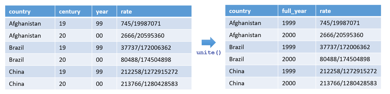
6.6.2 Combining Columns with unite()

Conversely, the unite() function merges multiple columns into one.

Figure 6.5: Combining Multiple Columns into One Using unite()

Its syntax is:

unite(data, col = <name of new column>, ..., sep = <separator>, remove = <logical flag>)

Where:

• data: The data frame to be transformed.

• col: The name of the new column that will contain the combined values.

• ...: The columns to combine.

• sep: The separator to insert between values (defaults to "_" if not specified).

• remove: A logical flag (default TRUE) indicating whether to remove the original columns after merging.

Example 2:

Imagine your TB dataset has separate "century" and "year" columns that you want to combine into a single "year" column:

# Create the data frame
tb_cases <- tibble(
  country = c("Afghanistan", "Afghanistan", "Brazil", "Brazil", "China", "China"),
  century = c("19", "20", "19", "20", "19", "20"),
  year = c("99", "00", "99", "00", "99", "00"),
  rate = c("745/19987071", "2666/20595360", "37737/172006362", "80488/174504898", "212258/1272915272", "213766/1280428583")
)

tb_cases

#> # A tibble: 6 × 4
#>   country     century year  rate             
#>   <chr>       <chr>   <chr> <chr>            
#> 1 Afghanistan 19      99    745/19987071     
#> 2 Afghanistan 20      00    2666/20595360    
#> 3 Brazil      19      99    37737/172006362  
#> 4 Brazil      20      00    80488/174504898  
#> 5 China       19      99    212258/1272915272
#> 6 China       20      00    213766/1280428583

You can merge "century" and "year" into a single column, also named "year", by specifying no separator:

tb_cases |> unite(year, century, year, sep = "")

#> # A tibble: 6 × 3
#>   country     year  rate             
#>   <chr>       <chr> <chr>            
#> 1 Afghanistan 1999  745/19987071     
#> 2 Afghanistan 2000  2666/20595360    
#> 3 Brazil      1999  37737/172006362  
#> 4 Brazil      2000  80488/174504898  
#> 5 China       1999  212258/1272915272
#> 6 China       2000  213766/1280428583

Important

This operation tidies your dataset by reducing two related columns into one, making future analysis more straightforward.

6.6.3 Practice Quiz 6.2

Question 1:

Given the following tibble:

tb_cases <- tibble(
  country = c("Brazil", "Brazil", "China", "China"),
  year = c(1999, 2000, 1999, 2000),
  rate = c("37737/172006362", "80488/174504898", "212258/1272915272", "213766/1280428583")
)

Which function would you use to split the "rate" column into two separate columns for cases and population?

1. separate()
   
2. unite()
   
3. pivot_longer()
   
4. pivot_wider()

Question 2:

Which argument in separate() allows automatic conversion of new columns to appropriate data types?

1. remove
   
2. auto
3. convert
4. into

Question 3:

Which function would you use to merge two columns into one, for example, combining separate “century” and “year” columns?

1. separate()
   
2. unite()
   
3. pivot_longer()
   
4. pivot_wider()

Question 4:

In the separate() function, what does the sep argument define?

1. The new column names
   
2. The delimiter at which to split the column
   
3. The data frame to be merged
   
4. The columns to remove

Question 5:

Consider the following data frame:

tb_cases <- tibble(
  country = c("Afghanistan", "Brazil", "China"),
  century = c("19", "19", "19"),
  year = c("99", "99", "99")
)

Which code correctly combines “century” and “year” into a single column “year” without any separator?

1. tb_cases |> unite(year, century, year, sep = "")
   
2. tb_cases |> separate(year, into = c("century", "year"), sep = "")
   
3. tb_cases |> unite(year, century, year, sep = "_")
   
4. tb_cases |> pivot_longer(cols = c(century, year))

Question 6:

When using separate(), how can you retain the original column after splitting it?

1. Set remove = FALSE
   
2. Set convert = TRUE
   
3. Use unite() instead
   
4. Omit the sep argument

Question 7:

Which variant of separate() would you use to split a column at fixed character positions?

1. separate_wider_delim()
   
2. separate_wider_regex()
   
3. separate_wider_position()
   
4. separate()

Question 8:

By default, the unite() function removes the original columns after combining them.

1. True
   
2. False

Question 9:

What is the main benefit of using separate() on a column that combines multiple data points (e.g. “745/19987071”)?

1. It facilitates the conversion of string data into numeric data automatically.
   
2. It simplifies further analysis by splitting combined information into distinct, analysable components.
   
3. It merges the data with another dataset.
   
4. It increases data redundancy.

Question 10:

Which argument in unite() determines the character inserted between values when combining columns?

1. separator
   
2. sep
   
3. col
   
4. delimiter

See the Solution to Quiz 6.2

6.6.4 Exercise 6.2.1: Transforming the Television Company Dataset

This exercise tests your data cleaning skills using the television-company-data.csv dataset, which can be found in the r-data directory. If you do not already have the file, you may download it from Google Drive.

Dataset Metadata

This dataset was gathered by a small television company aiming to understand the factors influencing viewer ratings of the company. It contains viewer ratings and related metrics. The variables are as follows:

• regard: Viewer rating of the television company (higher ratings indicate greater regard).

• gender: The gender with which the viewer identifies.

• views: The number of views.

• online: The number of times bonus online material was accessed.

• library: The number of times the online library was browsed.

• Shows: Scores for four different shows, each separated by a comma.

Tasks

1. Importing and Inspecting Data

   • Locate the television-company-data.csv file in the r-data directory.

   • Import the data into your R environment.

2. Data Tidying

   • Create four new columns from the Shows column, naming them Show1 through Show4.

   • Create a new variable, mean_show, calculated as the mean of Show1 to Show4.

   • Examine how the mean show scores vary by gender.

See the Solution to Exercise 6.2.1

6.7 Experiment 6.3: Combining Datasets with Joins

When you’re working with real-world data, it’s common to have information scattered across multiple tables. In order to get a full picture and answer the questions you are interested in, you often need to merge these datasets. In this section, we will dive into how you can accomplish this in R using joins, a fundamental concept in both database management and data analysis.

6.7.1 The Role of Keys

Before you begin joining datasets, it’s crucial to understand what keys are and why they matter. In relational databases, a key is a column (or set of columns) that uniquely identifies each row in your dataset. When you join tables, keys determine how rows are matched across your datasets.

• Primary Key: Think of this as the unique identifier for each record in a table. For example, in students table (Table 6.3 (a)), the student_id is the primary key because it uniquely identifies each student.

• Foreign Key: This is a column in another table that links back to the primary key of the first table. In our case, the student_id in an exam scores table (Table 6.3 (b)) would act as a foreign key, connecting scores to the corresponding students.

To illustrate, consider these two datasets in Table 6.3:

Table 6.3: Relational Keys in Action: Linking Datasets with Primary and Foreign Keys

(a) Students Table

student_id	name	age
1	Alice	20
2	Bob	22
3	Charlie	21

(b) Exam Scores Table

student_id	score
1	85
2	90
4	78

In the Students table, the student_id column is the primary key that uniquely identifies each student. In the Exam Scores table, student_id is used as a foreign key to refer back to the Students table. We will use these two tables to illustrate the different types of joins.

6.7.2 Types of Joins

Joins are the backbone of relational data analysis, and the dplyr offers a family of join functions to merge tables, each with a specific way of handling matches and non-matches. They all follow a similar pattern:

join_function(x, y, by = "key_column")

Where:

• x: The first table (the “left” table).

• y: The second table (the “right table”).

• by: The column(s) to match on.

Let’s explore the main types: inner, left, right, and full joins. We wll use students and scores to see how each one works.

6.7.2.1 Inner Join

An inner join keeps only the rows where the key matches in both tables. If there’s no match, the row gets dropped. It’s the strictest join—think of it as finding the overlap between two circles in a Venn diagram.

The syntax is:

inner_join(x, y, by = "key_column")

Example 1: Matching Students and Scores

Suppose you are a teacher who only wants to see data for students who are enrolled and took the exam. Using Tables 6.3 (a) and 6.3 (b):

students <- data.frame(student_id = 1:3, name = c("Alice", "Bob", "Charlie"), age = 20:22)

scores <- data.frame(student_id = c(1, 2, 4), score = c(85, 90, 78))

# Inner join
students |> inner_join(scores, by = "student_id")

#>   student_id  name age score
#> 1          1 Alice  20    85
#> 2          2   Bob  21    90

Tip

What’s Happening:

• Alice (student_id 1) and Bob (student_id 2) appear because they’re in both tables.

• Charlie (student_id 3) is missing—he didn’t take the exam, so there’s no match in scores.

• Student_id 4 is also out—it’s in scores but not students.

This join is perfect when you need complete data from both sides, like calculating averages for students with scores.

Note

Think about how the result might change if we used left_join() instead?

6.7.2.2 The Left Join

A left join keeps every row from the left table (x) and brings along matching rows from the right table (y). If there’s no match, you get NA in the columns from y.

The syntax is:

left_join(x, y, by = "key_column")

Example 2: Report Cards for All Students

Imagine you are preparing report cards and need every student listed, even if they missed the exam:

# Left join
students |> left_join(scores, by = "student_id")

#>   student_id    name age score
#> 1          1   Alice  20    85
#> 2          2     Bob  21    90
#> 3          3 Charlie  22    NA

Tip

What’s Happening:

• All three students from students are here because it’s the left table.

• Alice and Bob have their scores (85 and 90).

• Charlie gets an NA for score—he’s enrolled but didn’t take the test.

• Student_id 4 from scores is excluded—it’s not in the left table.

Use this when the left table is your priority, like ensuring every student gets a report card.

Warning

Consider what happens if the id column contains duplicates in either df1 or df2. This could result in more rows than expected in the joined dataset.

6.7.2.3 The Right Join

A right join flips it around: it keeps all rows from the right table (y) and matches them with the left table (x), filling in NA where needed.

The syntax is:

right_join(x, y, by = "key_column")

Example 3: All Exam Scores

Now, suppose the exam office wants every score reported, even for students not in your class list:

# Right join

students |> right_join(scores, by = "student_id")

#>   student_id  name age score
#> 1          1 Alice  20    85
#> 2          2   Bob  21    90
#> 3          4  <NA>  NA    78

Tip

What’s Happening:

• All three scores from scores are included because it’s the right table.

• Alice and Bob match up with their info from students.

• Student_id 4 has a score (78) but no name or age (NA)—they’re not in students.

This is handy when the right table drives the analysis, like auditing all exam results.

6.7.2.4 The Full Join

A full join keeps everything—every row from both tables, matching where possible and using NA for gaps. It’s the most inclusive join.

The syntax is:

full_join(x, y, by = "key_column")

Example 4: Complete Audit

For an audit, you want every student and every score, matched or not:

# Full join

students |> full_join(scores, by = "student_id")

#>   student_id    name age score
#> 1          1   Alice  20    85
#> 2          2     Bob  21    90
#> 3          3 Charlie  22    NA
#> 4          4    <NA>  NA    78

Tip

What’s Happening:

• Every student_id from both tables is here.

• Alice and Bob are fully matched.

• Charlie has no score (NA in score).

• Student_id 4 has a score but no student info (NA in name and age).

This join is your go-to when you can’t afford to lose any data, like reconciling records.

6.7.3 Joins with Different Key Names

What happens when the keys don’t have the same name? Real datasets often throw this curveball—the primary key in one table might be club_code, while the foreign key in another is group_id. No worries—dplyr can still connect them.

Let’s try a new example:

clubs <- tibble(club_code = c("A01", "B02", "C03"), club_name = c("Chess Club", "Robotics Team", "Art Society"))

members <- tibble(member_id = 101:103, name = c("Alice", "Bob", "Charlie"), group_id = c("A01", "B02", "D04"))

Check them out:

clubs

#> # A tibble: 3 × 2
#>   club_code club_name    
#>   <chr>     <chr>        
#> 1 A01       Chess Club   
#> 2 B02       Robotics Team
#> 3 C03       Art Society

members

#> # A tibble: 3 × 3
#>   member_id name    group_id
#>       <int> <chr>   <chr>   
#> 1       101 Alice   A01     
#> 2       102 Bob     B02     
#> 3       103 Charlie D04

Here, club_code is the primary key in clubs, and group_id is the foreign key in members. They’re different names, but their values (like “A01” and “B02”) match up.

Example:

You are a club coordinator and want to see who’s in which club, despite the naming mismatch. Use an inner join with a named vector in by:

clubs |> inner_join(members, by = c("club_code" = "group_id"))

#> # A tibble: 2 × 4
#>   club_code club_name     member_id name 
#>   <chr>     <chr>             <int> <chr>
#> 1 A01       Chess Club          101 Alice
#> 2 B02       Robotics Team       102 Bob

Tip

What’s Happening:

• The by = c("club_code" = "group_id") tells R to match club_code from clubs with group_id from members.

• Alice (A01) and Bob (B02) match their clubs.

• Charlie (D04) is dropped—there’s no D04 in clubs.

This trick works with any join type. For instance, a full join would include Charlie and the unmatched C03 club:

clubs |> full_join(members, by = c("club_code" = "group_id"))

#> # A tibble: 4 × 4
#>   club_code club_name     member_id name   
#>   <chr>     <chr>             <int> <chr>  
#> 1 A01       Chess Club          101 Alice  
#> 2 B02       Robotics Team       102 Bob    
#> 3 C03       Art Society          NA <NA>   
#> 4 D04       <NA>                103 Charlie

Joins are your superpower for combining datasets in R. With inner_join(), you get the overlap; left_join() prioritizes the left table; right_join() favours the right; and full_join() keeps it all. Plus, you can handle differently named keys with a simple tweak to by.

6.7.4 Practice Quiz 6.3

Question 1:

Given the following data frames:

df1 <- data.frame(id = 1:4, name = c("Ezekiel", "Bob", "Samuel", "Diana"))

df2 <- data.frame(id = c(2, 3, 5), score = c(85, 90, 88))

Which join would return only the rows with matching id values in both data frames?
a) left_join()
b) right_join()
c) inner_join()
d) full_join()

Question 2:

Using the same data frames, which join function retains all rows from df1 and fills unmatched rows with NA?

1. left_join()
   
2. inner_join()
   
3. right_join()
   
4. full_join()

Question 3:

Which join function ensures that all rows from df2 are preserved, regardless of matches in df1?

1. left_join()
   
2. inner_join()
   
3. full_join()
4. right_join()

Question 4:

What does a full join return when applied to df1 and df2?

1. Only matching rows
   
2. All rows from both data frames, with NA for unmatched entries
   
3. Only rows from df1
   
4. Only rows from df2

Question 5:

In a join operation, what is the purpose of the by argument?

1. It specifies the common column(s) used to match rows between the data frames
   
2. It orders the data frames
   
3. It selects which rows to retain
   
4. It converts keys to numeric values

Question 6:

If df1 contains duplicate values in the key column, what is a likely outcome of an inner join with df2?

1. The joined data frame may contain more rows than either original data frame due to duplicate matches.
   
2. The join will remove all duplicates automatically.
   
3. The function will return an error.
   
4. The duplicate rows will be merged into a single row.

Question 7:

An inner join returns all rows from both data frames, regardless of whether there is a match.

1. True
   
2. False

Question 8:

Consider the following alternative key columns:

df1 <- data.frame(studentID = 1:4, name = c("Alice", "Bob", "Charlie", "Diana"))

df2 <- data.frame(id = c(2, 3, 5), score = c(85, 90, 88))

How can you join these two data frames when the key column names differ?

1. Rename one column before joining.
   
2. Use by = c("studentID" = "id") in the join function.
3. Use an inner join without specifying keys.
   
4. Convert the keys to factors.

Question 9:

What is a ‘foreign key’ in the context of joining datasets?

1. A column in one table that uniquely identifies each row.
   
2. A column in one table that refers to the primary key in another table.
3. A column that has been split into multiple parts.
   
4. A column that is combined using unite().

Question 10:

Which join function would be most appropriate if you want a complete union of two datasets, preserving all rows from both?

1. full_join()
2. inner_join()
   
3. left_join()
   
4. right_join()

See the Solution to Quiz 6.3

6.7.5 Exercise 6.3.1: Relational Analysis with the NYC Flights 2013 Dataset

This exercise tests your relational analysis skills using the nycflights13 dataset, which is available as an R package. To access it, install and load the package.

Dataset Metadata

The nycflights13 dataset contains information on all 336,776 outbound flights from New York City airports (Newark Liberty International Airport (EWR), John F. Kennedy International Airport (JFK) and LaGuardia Airport (LGA)) in 2013, compiled from various sources, including the U.S. Bureau of Transportation Statistics. It is designed to explore the relationships between flight details, aircraft information, airport data, weather conditions and airline carriers. The dataset comprises five main tables:

• flights: Details of each flight, including departure and arrival times, delays and identifiers such as tailnum (aircraft tail number), origin (departure airport), dest (destination airport) and carrier (airline code). This table contains 336,776 rows and 19 columns.

• planes: Information about aircraft, such as the manufacturer, model and year built, linked by the tailnum key. This table contains 3,322 rows and 9 columns.

• airports: Data on airports, including location and name, linked by the faa code (used in flights$origin and flights$dest). This table contains 1,458 rows and 8 columns.

• weather: Hourly weather data for New York City airports, linked by origin and time_hour. This table contains 26,115 rows and 15 columns.

• airlines: Airline names and their carrier codes, linked by carrier. This table contains 16 rows and 2 columns.

Tasks

1. Importing and Inspecting Data

   • Install and load the nycflights13 package in your R environment.

   • Access the flights and planes tables, and inspect their structure to familiarise yourself with their variables.

   • Identify the common key (tailnum) that links flights and planes, and note any potential mismatches (for example, flights without corresponding plane data).

2. Relational Analysis with Joins

   • Perform an inner_join between flights and planes using the tailnum key. How many rows are in the result, and why might this differ from the number of rows in flights?

   • Perform a left_join between flights and planes using the tailnum key. Compare the number of rows with the original flights table, and explain what happens to flights without matching plane data.

   • Perform a right_join between flights and planes using the tailnum key. How does this differ from the left_join result, and what does it reveal about planes not used in flights?

   • Perform a full_join between flights and planes using the tailnum key. Describe how this result combines information from both tables, including cases with no matches.

   • Create a summary table showing the number of flights per aircraft manufacturer (from planes$manufacturer) after performing a left_join. Handle missing values appropriately (for example, label flights with no plane data as “Unknown”).

   • Produce a bar plot to visualise the distribution of flights across the top five aircraft manufacturers based on your summary table.

Happy joining!

See the Solution to Exercise 6.3.1

6.8 Reflective Summary

In Lab 6, you have acquired advanced data transformation skills essential for effective data analysis:

• Reshaping Data: You learned to convert datasets between wide and long formats using pivot_longer() and pivot_wider(). Mastering these techniques is foundational for conducting time series analyses and creating visualisations.

• Separating and Uniting Columns: You explored how to split a single column into multiple columns with separate() and combine several columns into one with unite(), thereby enhancing the structure of your data.

• Combining Datasets: You became familiar with various join operations in dplyr, enabling you to merge datasets seamlessly and manage issues such as mismatched keys and duplicates.

What’s Next?

In the next lab, we will delve into data visualisation where will transform raw data into a visual language that reveals patterns, highlights trends, and conveys stories in ways that are easy to understand and interpret.