11  Use Case Projects

11.1 Introduction

In previous labs, you learned how to organise workflows, transform data, create visualisations, and contextualise your technical skills within the broader field of data science. Lab 11 takes this learning further by emphasising the power of applying your skills to realistic, end-to-end projects. Engaging in use case projects bridges the gap between theory and practice, allowing you to internalise concepts, strengthen problem-solving abilities, and gain invaluable experience.

11.2 Learning Objectives

By the end of this lab, you will be able to:

• Integrate Previously Learned Skills into Practical Projects
  Combine data wrangling, visualisation, reproducibility, and statistical techniques to solve real-world problems.

• Improve Problem-Solving Through Iterative Practice
  Gain the ability to troubleshoot, adapt, and refine your approach in response to unexpected challenges in data analysis.

• Develop a Holistic Understanding of Workflows
  Recognise how each stage of the data analysis process—importing data, cleaning, transforming, modelling, and communicating—fits into a cohesive project.

• Build Confidence and Portfolios
  Complete projects that demonstrate your proficiency, increasing self-assurance and providing tangible evidence of your capabilities.

• Communicate Findings Effectively
  Present insights, methods, and recommendations through clear reporting and visualisations, ensuring results can guide informed decisions.

By completing this lab, you’ll deepen your understanding of R and data analysis methodologies by tackling real-world scenarios. This hands-on approach cements your learning, enhances creativity, boosts confidence, and helps you build a portfolio of projects that can showcase your capabilities to employers, colleagues, and mentors.

11.3 Prerequisites

Before starting this lab, you should have:

• Completed Labs 1–9, gaining familiarity with setting up R projects, transforming data, visualising information, understanding the data science lifecycle, and contextualising your technical skills.

• Basic understanding of statistical concepts, data wrangling, reproducible workflows, and visualisation techniques.

• An interest in applying your learned skills to realistic scenarios, moving beyond isolated exercises and theoretical discussions.

11.4 Why Use Case Projects?

While earlier labs focused on mastering individual techniques, use case projects show how these techniques fit together in solving a real-world problem. This approach:

1. Application of Theory: Practical projects allow learners to apply the theoretical knowledge they’ve acquired. This transition from theory to application often solidifies understanding.

2. Problem-Solving Skills: Real-world projects present unforeseen challenges. By working through these, learners enhance their problem-solving skills and become adept at troubleshooting.

3. Comprehensive Understanding: Use case projects often require the integration of various R functions and techniques. This holistic approach ensures a deeper and more comprehensive grasp of R.

4. Confidence Building: Successfully completing a use-case project boosts confidence, giving students the assurance that they can tackle real-world data problems using R.

5. Portfolio Building: Adds substantial examples of your work for future presentations or job applications.

Reflection Question

How does applying your skills in a realistic project setting differ from learning them in isolation, and why might this approach lead to deeper mastery?

11.5 Use Case 1: Telco Customer Churn Data Analysis and Visualization Assessment

You have been provided with the Telco Customer Churn dataset, which includes detailed information on customer demographics, account details, subscribed services, and churn behaviour. Your task is to leverage your R skills to transform, analyse, and visualise this data, generating actionable insights. Synthesize your findings into a concise report to communicate key patterns, trends, and recommendations.

Dataset Overview

The Telco Customer Churn dataset provides comprehensive details about customers, including their demographics, account information, service usage, and whether they have churned. Key columns include:

• customerID: Unique identifier for each customer.

• gender: Customer gender (‘Male’ or ‘Female’).

• SeniorCitizen: Indicator if the customer is a senior (1 for Yes, 0 for No).

• Partner: Whether the customer has a partner (‘Yes’ or ‘No’).

• Dependents: Whether the customer has dependents (‘Yes’ or ‘No’).

• tenure: Number of months the customer has stayed with the company.

• PhoneService: Indicates if the customer has a phone service (‘Yes’ or ‘No’).

• MultipleLines: Indicates if the customer has multiple phone lines (‘Yes’, ‘No’, or ‘No phone service’).

• InternetService: Type of internet service (‘DSL’, ‘Fiber optic’, or ‘No’).

• OnlineSecurity, OnlineBackup, DeviceProtection, TechSupport, StreamingTV, StreamingMovies: Service-specific columns with values (‘Yes’, ‘No’, or ‘No internet service’).

• Contract: Customer’s contract type (‘Month-to-month’, ‘One year’, or ‘Two year’).

• PaperlessBilling: Whether the customer uses paperless billing (‘Yes’ or ‘No’).

• PaymentMethod: Customer’s payment method (e.g., ‘Electronic check’, ‘Mailed check’, ‘Bank transfer (automatic)’, ‘Credit card (automatic)’).

• MonthlyCharges: Amount charged to the customer monthly.

• TotalCharges: Total amount charged to the customer.

• Churn: Indicates whether the customer has churned (‘Yes’ or ‘No’).

For full metadata, see sheet 2 of the telco-customer-churn.xlsx file or visit Kaggle.

Tasks

1. Data Manipulation and Transformation

   1. Data Import:
      • Locate and import the Telco Customer Churn data (telco-customer-churn.xlsx) from the r-data directory. If you do not already have the file, you can download it from Google Drive.
   2. Variable Transformation:

      • Transform the Churn column into a binary format (e.g., 1 for churned, 0 for not churned).

      • Recode the SeniorCitizen variable into a more descriptive format (e.g., “Yes” for 1 and “No” for 0).
        

      • Create a new variable, such as AvgChargePerMonth, calculated by dividing TotalCharges by tenure (ensuring that cases where tenure is 0 are handled appropriately).

      • Optionally, develop another metric (e.g., a ServiceCount that aggregates the number of additional services to which a customer subscribes).

2. Handling Missing and Inconsistent Values

   1. Identify Issues:
      • Scan the dataset for missing or inconsistent values, and document which columns are affected.
   2. Data Quality Improvement:
      • Apply strategies to address any data quality issues (for example, convert data types if necessary, handle missing values, and ensure consistency across columns).

3. Analysis and Insights

   1. Overall Churn Patterns:
      • Determine the overall churn rate in the dataset.
   2. Segmented Analysis:

      • Calculate the percentage of churned customers across different segments such as:

        • Gender: What proportion of male vs. female customers churn?

        • Contract Type: How does the churn rate vary across different contract types?

        • Internet Service: What are the churn rates for customers with DSL, Fiber optic, or no internet service?

      • For each segment (or combination of segments), compute summary statistics (e.g., counts, averages, medians) for key metrics like MonthlyCharges and tenure.

   3. Advanced Aggregation:

      • For each gender, determine summary statistics (mean, median, maximum) for monthly charges.

      • Identify which customer segment or service bundle is associated with the highest churn rate.

4. Data Visualization

   1. Exploratory Visualizations:

      • Create a histogram or density plot to visualize the distribution of customer tenure.

      • Develop a bar chart that shows the counts of churned and non-churned customers.

   2. Comparative Visualizations:

      • Construct a boxplot to compare MonthlyCharges across different Contract types.

      • Generate a scatter plot displaying the relationship between tenure and MonthlyCharges, with points colored by churn status. Consider adding a trend line if it enhances interpretation.

   3. Combined Analysis:

      • Filter the dataset to focus on a specific segment (for example, only customers with ‘Fiber optic’ service) and create additional visualizations (such as a histogram of their tenure or a scatter plot of their charges vs. tenure).

      • For each unique tenure value, compute the percentage of customers who churned, and plot these percentages as a line graph.

Deliverables

• Code:
  Provide your R script or R Markdown file with clear, commented code showing your data manipulation, analysis, and visualization steps.

• Report:
  Write a concise summary that explains:

  • Your approach to data cleaning and transformation.
  • The key findings from your analysis.
  • Insights derived from your visualizations.
  • Any recommendations or follow-up questions that your analysis suggests.

11.6 Use Case 1: The Solution

This document analyses the Telco Customer Churn dataset. It covers data import, transformation, analysis, and visualisation.

Data Manipulation and Transformation

Data Import and Initial Exploration

We begin by loading the required libraries and importing the data.

# Load required libraries
library(tidyverse) # For data manipulation and visualisation
library(readxl) # For data import
library(inspectdf) # For inspecting missing values

# Set the file path for the Telco Customer Churn dataset
file_path <- "r-data/telco-customer-churn.xlsx"

# Read the spreadsheet file into a tibble
telco <- read_xlsx(file_path, sheet = 1)

# Explore the dataset structure, summary statistics, and first few     rows
glimpse(telco)

#> Rows: 2,110
#> Columns: 21
#> $ customer_id       <chr> "1452-KIOVK", "6388-TABGU", "9763-GRSKD", "3655-SNQY…
#> $ gender            <chr> "Male", "Male", "Male", "Female", "Male", "Female", …
#> $ senior_citizen    <dbl> 0, 0, 0, 0, 0, 0, 0, 0, 0, 0, 0, 0, 0, 0, 0, 0, 1, 0…
#> $ partner           <chr> "No", "No", "Yes", "Yes", "No", "Yes", "Yes", "Yes",…
#> $ dependents        <chr> "Yes", "Yes", "Yes", "Yes", "Yes", "Yes", "Yes", "Ye…
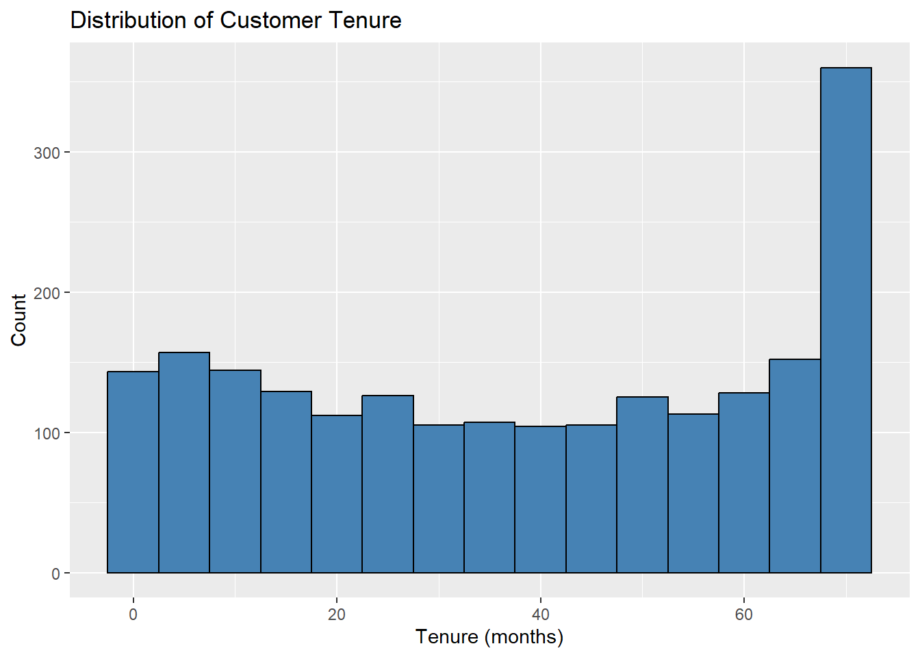
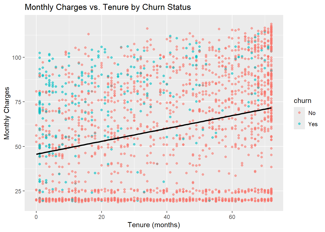
#> $ tenure            <dbl> 22, 62, 13, 69, 71, 10, 49, 47, 1, 17, 27, 72, 10, 7…
#> $ phone_service     <chr> "Yes", "Yes", "Yes", "Yes", "Yes", "Yes", "Yes", "Ye…
#> $ multiple_lines    <chr> "Yes", "No", "No", "Yes", "Yes", "No", "No", "Yes", …
#> $ internet_service  <chr> "Fiber optic", "DSL", "DSL", "Fiber optic", "Fiber o…
#> $ online_security   <chr> "No", "Yes", "Yes", "Yes", "Yes", "No", "Yes", "No",…
#> $ online_backup     <chr> "Yes", "Yes", "No", "Yes", "No", "No", "Yes", "Yes",…
#> $ device_protection <chr> "No", "No", "No", "Yes", "Yes", "Yes", "No", "No", "…
#> $ tech_support      <chr> "No", "No", "No", "Yes", "No", "Yes", "Yes", "No", "…
#> $ streaming_tv      <chr> "Yes", "No", "No", "Yes", "Yes", "No", "No", "Yes", …
#> $ streaming_movies  <chr> "No", "No", "No", "Yes", "Yes", "No", "No", "Yes", "…
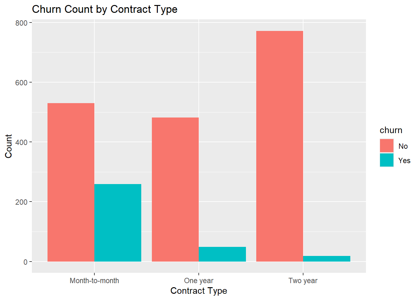
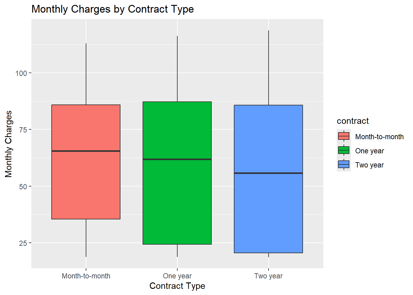
#> $ contract          <chr> "Month-to-month", "One year", "Month-to-month", "Two…
#> $ paperless_billing <chr> "Yes", "No", "Yes", "No", "No", "No", "No", "Yes", "…
#> $ payment_method    <chr> "Credit card (automatic)", "Bank transfer (automatic…
#> $ monthly_charges   <dbl> 89.10, 56.15, 49.95, 113.25, 106.70, 55.20, 59.60, 9…
#> $ total_charges     <chr> "1949.4", "3487.95", "587.45000000000005", "7895.15"…
#> $ churn             <chr> "No", "No", "No", "No", "No", "Yes", "No", "Yes", "Y…

summary(telco)

#>  customer_id           gender          senior_citizen      partner         
#>  Length:2110        Length:2110        Min.   :0.00000   Length:2110       
#>  Class :character   Class :character   1st Qu.:0.00000   Class :character  
#>  Mode  :character   Mode  :character   Median :0.00000   Mode  :character  
#>                                        Mean   :0.04313                     
#>                                        3rd Qu.:0.00000                     
#>                                        Max.   :1.00000                     
#>   dependents            tenure      phone_service      multiple_lines    
#>  Length:2110        Min.   : 0.00   Length:2110        Length:2110       
#>  Class :character   1st Qu.:16.00   Class :character   Class :character  
#>  Mode  :character   Median :39.00   Mode  :character   Mode  :character  
#>                     Mean   :38.37                                        
#>                     3rd Qu.:62.00                                        
#>                     Max.   :72.00                                        
#>  internet_service   online_security    online_backup      device_protection 
#>  Length:2110        Length:2110        Length:2110        Length:2110       
#>  Class :character   Class :character   Class :character   Class :character  
#>  Mode  :character   Mode  :character   Mode  :character   Mode  :character  
#>                                                                             
#>                                                                             
#>                                                                             
#>  tech_support       streaming_tv       streaming_movies     contract        
#>  Length:2110        Length:2110        Length:2110        Length:2110       
#>  Class :character   Class :character   Class :character   Class :character  
#>  Mode  :character   Mode  :character   Mode  :character   Mode  :character  
#>                                                                             
#>                                                                             
#>                                                                             
#>  paperless_billing  payment_method     monthly_charges  total_charges     
#>  Length:2110        Length:2110        Min.   : 18.70   Length:2110       
#>  Class :character   Class :character   1st Qu.: 24.50   Class :character  
#>  Mode  :character   Mode  :character   Median : 60.98   Mode  :character  
#>                                        Mean   : 59.52                     
#>                                        3rd Qu.: 85.95                     
#>                                        Max.   :118.75                     
#>     churn          
#>  Length:2110       
#>  Class :character  
#>  Mode  :character  
#>                    
#>                    
#> 

head(telco)

#> # A tibble: 6 × 21
#>   customer_id gender senior_citizen partner dependents tenure phone_service
#>   <chr>       <chr>           <dbl> <chr>   <chr>       <dbl> <chr>        
#> 1 1452-KIOVK  Male                0 No      Yes            22 Yes          
#> 2 6388-TABGU  Male                0 No      Yes            62 Yes          
#> 3 9763-GRSKD  Male                0 Yes     Yes            13 Yes          
#> 4 3655-SNQYZ  Female              0 Yes     Yes            69 Yes          
#> 5 9959-WOFKT  Male                0 No      Yes            71 Yes          
#> 6 4190-MFLUW  Female              0 Yes     Yes            10 Yes          
#> # ℹ 14 more variables: multiple_lines <chr>, internet_service <chr>,
#> #   online_security <chr>, online_backup <chr>, device_protection <chr>,
#> #   tech_support <chr>, streaming_tv <chr>, streaming_movies <chr>,
#> #   contract <chr>, paperless_billing <chr>, payment_method <chr>,
#> #   monthly_charges <dbl>, total_charges <chr>, churn <chr>

# Inspect missing values for each column
telco %>%
  inspect_na() %>%
  print(n = 21)

#> # A tibble: 21 × 3
#>    col_name            cnt  pcnt
#>    <chr>             <int> <dbl>
#>  1 total_charges        11 0.521
#>  2 customer_id           0 0    
#>  3 gender                0 0    
#>  4 senior_citizen        0 0    
#>  5 partner               0 0    
#>  6 dependents            0 0    
#>  7 tenure                0 0    
#>  8 phone_service         0 0    
#>  9 multiple_lines        0 0    
#> 10 internet_service      0 0    
#> 11 online_security       0 0    
#> 12 online_backup         0 0    
#> 13 device_protection     0 0    
#> 14 tech_support          0 0    
#> 15 streaming_tv          0 0    
#> 16 streaming_movies      0 0    
#> 17 contract              0 0    
#> 18 paperless_billing     0 0    
#> 19 payment_method        0 0    
#> 20 monthly_charges       0 0    
#> 21 churn                 0 0

Data Cleaning and Transformation

We transform the churn column into a binary indicator, recode senior_citizen, and create a new variable service_count to count additional service subscriptions.

# Transform Churn to a binary indicator and recode SeniorCitizen for     clarity
telco <- telco %>%
  mutate(
    churn_binary = if_else(churn == "Yes", 1, 0),
    senior_citizen = if_else(senior_citizen == 1, "Yes", "No")
  )

# Create a ServiceCount variable to sum additional service     subscriptions
telco <- telco %>%
  mutate(
    phone_service_flag = if_else(phone_service == "Yes", 1, 0),
    online_security_flag = if_else(online_security == "Yes", 1, 0),
    online_backup_flag = if_else(online_backup == "Yes", 1, 0),
    device_protection_flag = if_else(device_protection == "Yes", 1, 0),
    tech_support_flag = if_else(tech_support == "Yes", 1, 0),
    streaming_tv_flag = if_else(streaming_tv == "Yes", 1, 0),
    streaming_movies_flag = if_else(streaming_movies == "Yes", 1, 0),
    service_count = phone_service_flag + online_security_flag + online_backup_flag +
      device_protection_flag + tech_support_flag + streaming_tv_flag +
      streaming_movies_flag
  ) %>%
  # Remove temporary flag columns for cleanliness
  select(-ends_with("_flag"))

Recoding Additional Demographic and Payment Variables

Recode key demographic variables to enhance interpretability and group similar payment methods.

# Recode SeniorCitizen into SeniorStatus
telco <- telco %>%
  mutate(senior_status = if_else(senior_citizen == "Yes", "Senior", "Non-Senior"))

# Recode Partner into PartnerStatus
telco <- telco %>%
  mutate(partner_status = if_else(partner == "Yes", "Partner", "No Partner"))

# Recode Dependents into DependentStatus
telco <- telco %>%
  mutate(dependent_status = if_else(dependents == "Yes", "Dependents", "No Dependents"))

# Group PaymentMethod into broader categories
telco <- telco %>%
  mutate(
    payment_method_group = case_when(
      payment_method == "Electronic check" ~ "Electronic check",
      payment_method == "Mailed check" ~ "Mailed check",
      str_detect(payment_method, "automatic") ~ "Automatic",
      TRUE ~ payment_method # Catch-all for any unexpected values
    )
  )

# Convert all non-numeric columns (except customerID) to factors for clarity
telco <- telco %>%
  mutate(across(
    .cols = -customer_id, # Exclude customerID column
    .fns = ~ if (!is.numeric(.)) as.factor(.) else .
  ))

Analysis and Insights

Summarise Churn Rates by New Variables

The following summaries show how churn rates vary across demographic and payment groups.

# Churn rate by SeniorStatus
churn_by_senior <- telco %>%
  group_by(senior_status) %>%
  summarise(
    Count = n(),
    ChurnRate = mean(churn_binary, na.rm = TRUE) * 100
  )

churn_by_senior

#> # A tibble: 2 × 3
#>   senior_status Count ChurnRate
#>   <fct>         <int>     <dbl>
#> 1 Non-Senior     2019      15.1
#> 2 Senior           91      24.2

# Churn rate by PartnerStatus
churn_by_partner <- telco %>%
  group_by(partner_status) %>%
  summarise(
    Count = n(),
    ChurnRate = mean(churn_binary, na.rm = TRUE) * 100
  )

churn_by_partner

#> # A tibble: 2 × 3
#>   partner_status Count ChurnRate
#>   <fct>          <int>     <dbl>
#> 1 No Partner       361      21.3
#> 2 Partner         1749      14.2

# Churn rate by DependentStatus
churn_by_dependents <- telco %>%
  group_by(dependent_status) %>%
  summarise(
    Count = n(),
    ChurnRate = mean(churn_binary, na.rm = TRUE) * 100
  )

churn_by_dependents

#> # A tibble: 1 × 3
#>   dependent_status Count ChurnRate
#>   <fct>            <int>     <dbl>
#> 1 Dependents        2110      15.5

# Churn rate by PaymentMethodGroup
churn_by_payment <- telco %>%
  group_by(payment_method_group) %>%
  summarise(
    count = n(),
    avg_monthly_charges = mean(monthly_charges, na.rm = TRUE),
    churn_rate = mean(churn_binary, na.rm = TRUE) * 100
  )

churn_by_payment

#> # A tibble: 3 × 4
#>   payment_method_group count avg_monthly_charges churn_rate
#>   <fct>                <int>               <dbl>      <dbl>
#> 1 Automatic             1068                63.5       9.93
#> 2 Electronic check       479                73.6      32.2 
#> 3 Mailed check           563                40.0      11.7

Additional Data Analysis

We further explore churn rates across overall, contract, and internet service segments, as well as summarise monthly charges by gender.

# Overall churn rate
overall_churn_rate <- telco %>%
  summarise(
    Total = n(),
    churned = sum(churn_binary, na.rm = TRUE),
    churn_rate = churned / Total * 100
  )

overall_churn_rate

#> # A tibble: 1 × 3
#>   Total churned churn_rate
#>   <int>   <dbl>      <dbl>
#> 1  2110     326       15.5

# Churn rate by Contract Type
churn_by_contract <- telco %>%
  group_by(contract) %>%
  summarise(
    count = n(),
    avg_monthly_charges = mean(monthly_charges, na.rm = TRUE),
    avg_tenure = mean(tenure, na.rm = TRUE),
    churn_rate = mean(churn_binary, na.rm = TRUE) * 100
  )

churn_by_contract

#> # A tibble: 3 × 5
#>   contract       count avg_monthly_charges avg_tenure churn_rate
#>   <fct>          <int>               <dbl>      <dbl>      <dbl>
#> 1 Month-to-month   789                62.0       20.5      32.8 
#> 2 One year         531                60.6       40.9       9.23
#> 3 Two year         790                56.3       54.5       2.28

# Churn rate by Internet Service Type
churn_by_internet <- telco %>%
  group_by(internet_service) %>%
  summarise(
    count = n(),
    churnRate = mean(churn_binary, na.rm = TRUE) * 100
  )

churn_by_internet

#> # A tibble: 3 × 3
#>   internet_service count churnRate
#>   <fct>            <int>     <dbl>
#> 1 DSL                805     11.9 
#> 2 Fiber optic        662     30.5 
#> 3 No                 643      4.35

# Summary statistics for MonthlyCharges by Gender
charges_by_gender <- telco %>%
  group_by(gender) %>%
  summarise(
    mean_monthly_charges = mean(monthly_charges, na.rm = TRUE),
    median_monthly_charges = median(monthly_charges, na.rm = TRUE),
    max_monthly_charges = max(monthly_charges, na.rm = TRUE)
  )

charges_by_gender

#> # A tibble: 2 × 4
#>   gender mean_monthly_charges median_monthly_charges max_monthly_charges
#>   <fct>                 <dbl>                  <dbl>               <dbl>
#> 1 Female                 59.4                   61.2                119.
#> 2 Male                   59.6                   61.0                117.

# Identify Contract type with highest churn rate
highest_churn_contract <- churn_by_contract %>%
  arrange(desc(churn_rate))

highest_churn_contract

#> # A tibble: 3 × 5
#>   contract       count avg_monthly_charges avg_tenure churn_rate
#>   <fct>          <int>               <dbl>      <dbl>      <dbl>
#> 1 Month-to-month   789                62.0       20.5      32.8 
#> 2 One year         531                60.6       40.9       9.23
#> 3 Two year         790                56.3       54.5       2.28

Data Visualisation

Visualisations help uncover trends and patterns that might not be immediately apparent from summary tables.

Histogram of Customer Tenure

telco |> ggplot(aes(x = tenure)) +
  geom_histogram(binwidth = 5, fill = "steelblue", color = "black") +
  labs(title = "Distribution of Customer Tenure", x = "Tenure (months)", y = "Count")

Bar Chart of Churn Count by Contract Type

telco |> ggplot(aes(x = contract, fill = churn)) +
  geom_bar(position = position_dodge()) +
  labs(title = "Churn Count by Contract Type", x = "Contract Type", y = "Count")

Boxplot: MonthlyCharges across Contract Types

telco |> ggplot(aes(x = contract, y = monthly_charges, fill = contract)) +
  geom_boxplot() +
  labs(title = "Monthly Charges by Contract Type", x = "Contract Type", y = "Monthly Charges")

Scatter Plot: Tenure vs MonthlyCharges coloured by Churn Status

telco |> ggplot(aes(x = tenure, y = monthly_charges, color = churn)) +
  geom_point(alpha = 0.6) +
  geom_smooth(method = "lm", se = FALSE, color = "black") +
  labs(title = "Monthly Charges vs. Tenure by Churn Status", x = "Tenure (months)", y = "Monthly Charges")

#> `geom_smooth()` using formula = 'y ~ x'

Line Plot: Churn Rate by Tenure

churn_by_tenure <- telco %>%
  group_by(tenure) %>%
  summarise(
    Total = n(),
    Churned = sum(churn_binary, na.rm = TRUE),
    ChurnRate = Churned / Total * 100
  )

churn_by_tenure |> ggplot(aes(x = tenure, y = ChurnRate)) +
  geom_line(color = "darkred") +
  labs(title = "Churn Rate by Tenure", x = "Tenure (months)", y = "Churn Rate (%)")

Histogram: Tenure Distribution for Fibre Optic Customers

fiber_customers <- telco %>% filter(internet_service == "Fiber optic")

fiber_customers |> ggplot(aes(x = tenure)) +
  geom_histogram(binwidth = 5, fill = "darkgreen", color = "black") +
  labs(title = "Tenure Distribution for Fibre Optic Customers", x = "Tenure (months)", y = "Count")

Telco Customer Churn Analysis Report

Introduction

This report presents a comprehensive analysis of the Telco Customer Churn dataset, which contains detailed records of 7,043 customers. The dataset includes demographic information, account details, service usage metrics, and churn behaviour. Our primary objective is to identify key drivers of churn and develop actionable recommendations to improve customer retention. The analysis leverages robust data transformation, exploratory statistics, and visualisation techniques to uncover insights that can guide strategic decision-making.

Data Preparation and Transformation

Our initial steps focused on ensuring data quality and creating new variables to facilitate deeper insights. We:

• Cleaned the data by converting variables such as TotalCharges into a numeric format and recoding SeniorCitizen from a binary indicator into a descriptive format.

• Transformed the churn indicator into a binary variable (ChurnBinary), enabling precise calculation of churn rates.

• Derived new metrics like AvgChargePerMonth (TotalCharges divided by tenure) and ServiceCount (the total number of additional services a customer subscribes to).

• Re-encoded key demographic variables:

  • senior_status distinguishes between “Senior” and “Non-Senior” customers.
  • partner_status categorises customers as having a partner or not.
  • dependent_status identifies whether customers have dependents.

• Grouped payment methods into a new variable (payment_method_group) to compare broad categories: Automatic (including Bank transfer and Credit card), Electronic check, and Mailed check.

These transformations provided us with a richer dataset that supports more granular analyses of churn behaviour.

Exploratory Analysis and Key Findings

Overall Churn

Our analysis reveals an overall churn rate of approximately 26.5%. This indicates that about one in four customers leaves the service, underscoring the need for targeted retention strategies.

Contract Type and Internet Service

• Contract Type:
  • Customers on month-to-month contracts experience a markedly high churn rate of 42.7%.
    
  • In contrast, those on one-year and two-year contracts churn at rates of 11.3% and 2.8% respectively, suggesting that longer-term commitments are associated with greater customer loyalty.
• Internet Service:
  • Churn rates vary considerably by internet service type.
    
  • Fibre optic customers have a high churn rate of 41.9%, while DSL customers churn at 19.0%, and those with no internet service exhibit a relatively low churn rate of 7.4%.

These differences indicate that the type of service subscription plays a crucial role in customer retention. The high churn among fibre optic subscribers may reflect issues with pricing or service expectations.

Demographic Insights

• Senior Status:
  • Among Non-Seniors (5,901 customers), the churn rate is 23.6%.
    
  • In contrast, Seniors (1,142 customers) exhibit a significantly higher churn rate of 41.7%.
    
  • Interpretation: Seniors may face unique challenges or have different expectations that increase their propensity to leave.
• Partner Status:
  • Customers without a partner (3,641 customers) show a churn rate of 33.0%, while those with a partner (3,402 customers) churn at 19.7%.
    
  • Interpretation: Having a partner may indicate a more stable personal environment, which could translate into lower churn.
• Dependent Status:
  • Customers with dependents (2,110 customers) experience a churn rate of 15.5%, compared to 31.3% for those without dependents (4,933 customers).
    
  • Interpretation: The presence of dependents appears to be associated with a lower likelihood of churn, perhaps due to higher commitment levels or differing priorities.

Payment Methods

• Payment Method Group:
  • Customers paying via electronic check (2,365 customers) have the highest churn rate at 45.3% and also incur the highest average monthly charges (£76.3).
    
  • In contrast, those using automatic payment methods (3,066 customers) have a churn rate of 16.0% with an average monthly charge of £66.9, while mailed check users (1,612 customers) churn at 19.1% with lower average charges (£43.9).
    
  • Interpretation: The elevated churn rate among electronic check users might reflect higher costs or dissatisfaction with billing, indicating an area for potential intervention.

Visual Insights

Key visualisations further illustrate our findings:

• Tenure Distribution:
  A histogram of customer tenure reveals two distinct groups—new customers with very short tenures and a substantial cohort of long-term customers. This bimodal distribution suggests that retention strategies may need to be tailored differently for new versus established customers.

• Churn by Contract Type:
  Bar charts clearly show that month-to-month contracts drive the majority of churn, reinforcing the numerical findings.

• Monthly Charges vs. Tenure:
  A scatter plot demonstrates that customers with high monthly charges and short tenures are particularly prone to churn, highlighting the need for early intervention among this group.

• Churn Rate by Tenure:
  A line graph indicates that the churn rate declines steadily as tenure increases, emphasising the importance of retaining customers during the critical early months of service.

Recommendations

Based on these insights, we propose the following strategic recommendations:

1. Target Month-to-Month Subscribers:
   • Implement loyalty programmes or incentivise longer-term contracts to reduce the high churn rate in this segment.
2. Focus on Fibre Optic Subscribers:
   • Investigate the underlying causes of high churn among fibre optic users, such as pricing or service quality issues, and consider targeted offers to enhance value perception.
3. Enhanced Engagement for Senior Customers:
   • Develop tailored engagement initiatives for senior customers, who are significantly more likely to churn. This could include specialised support, personalised communication, or alternative service plans.
4. Review Payment Options:
   • Explore why customers using electronic checks are experiencing high churn and consider adjusting billing practices or offering alternative payment methods to improve satisfaction.
5. Early Intervention Strategies:
   • For new customers, especially those with high initial monthly charges, introduce proactive onboarding measures and personalised offers to encourage longer-term commitments.

Conclusion

The analysis indicates that while the overall churn rate stands at about 26.5%, particular customer segments—such as those on month-to-month contracts, fibre optic subscribers, senior customers, and users of electronic check payment methods—exhibit significantly higher churn rates. Addressing these vulnerabilities through targeted retention strategies and improved customer engagement will be crucial in reducing churn and enhancing long-term profitability.

11.7 Exercise 11.1: Analyzing a Rape Survey for the Federal Government of Nigeria

11.7.1 Project Overview

You have been engaged by the Federal Government of Nigeria to analyse a sensitive dataset about rape incidents gathered from a national survey in Lagos. Without explicit instructions, your task is to apply your data analysis and visualisation skills to uncover insights that may inform policy decisions, resource allocation, or awareness campaigns.

11.7.2 The Dataset

Locate the rape-survey.xlsx file in the r-data directory. If you don’t already have the file, you can download it from Google Drive.

11.7.3 Your Task

• Data Preparation: Import and clean the data, addressing missing values, verifying data formats, and ensuring variables align with analytical goals.

• Exploratory Analysis: Understand distributions of key variables, identify patterns or risk factors, and discover regional or demographic differences.

• Visualisation: Use bar charts, boxplots, or heatmaps to highlight differences among groups, time periods, or severity levels.

• Insights and Recommendations:
  Present findings in a concise, data-driven narrative. Consider ethical sensitivities when interpreting results. Provide recommendations that might guide policy, resource investment, or public education efforts.

11.8 Integrating Lab Skills

In previous labs, you learned how to organise projects (Lab 4), wrangle data (Lab 5 and Lab 6), visualise insights (Lab 7), and understand the broader data science field (Lab 10). Applying these techniques to real projects consolidates your skillset:

• Organisational Skills: Maintain reproducible workflows to ensure credibility and traceability.

• Data Wrangling: Tidy and transform datasets to facilitate smooth analysis and modelling.

• Visualisation: Create plots that reveal patterns, trends, or anomalies, guiding decision-makers effectively.

• Statistical and Analytical Rigor: Use tests and models judiciously, validating assumptions and ensuring insights are robust.

Note

Reflection Question

Having seen how individual techniques fit into larger projects, how does this perspective influence the way you approach learning new analytical methods or tools?

11.9 Conclusion and Further Steps

Use case projects are where R’s capabilities truly shine. By applying your skills to realistic scenarios, you cultivate problem-solving abilities, enhance creativity, and build confidence. Beyond academic exercises, these projects mirror professional tasks you might encounter in workplaces or research settings.

Next Steps:

• Continue seeking or designing new use case projects to keep skills sharp and current.

• Explore complex datasets, integrate more advanced modelling techniques, or experiment with interactive dashboards.

• Share your results publicly (in blogs, portfolios, or open-source contributions) to receive feedback and build a professional presence.

Note

Reflection Question:

As you move forward, what kind of real-world projects are you most interested in tackling, and how will these projects shape your future growth as a data professional?

11.10 General Practice Quiz 11

Question 1:

What is the main purpose of the pipe operator |> in R?

1. To run code in parallel.
   
2. To nest functions inside one another.
   
3. To pass the output of one function as the input to the next, improving code readability.
   
4. To automatically clean missing data.

Question 2:

In a reproducible R workflow (as discussed in early labs), which file type is commonly used to document code, results, and narrative together?

1. CSV files
   
2. R Markdown (or Quarto) documents
   
3. PNG images
   
4. Excel spreadsheets

Question 3:

When creating a new RStudio Project to ensure reproducibility and organisation of your analysis, what is one key advantage?

1. It automatically generates a machine learning model.
   
2. It sets the working directory to the project folder, simplifying relative paths.
   
3. It prevents all missing values.
   
4. It disables package installation from CRAN.

Question 4:

The principle of tidy data states that:

1. Each dataset should have no missing values.
   
2. Each column represents a variable, each row represents an observation, and each cell contains a single value.
   
3. Each dataset must have at least 10 columns.
   
4. Each value in the dataset must be numeric.

Question 5:

Which dplyr verb is used to filter rows based on logical conditions?

1. select()
   
2. mutate()
   
3. filter()
   
4. summarise()

Question 6:

To create new columns or modify existing ones in your dataset using dplyr, you would use:

1. select()
   
2. mutate()
   
3. arrange()
   
4. group_by()

Question 7:

Which ggplot2 component maps data variables to visual properties like axes, colour, or size?

1. Theme
   
2. Facets
   
3. Aesthetics (aes())
   
4. Scales

Question 8:

To reorder rows of data based on a variable’s value using dplyr, which function should be applied?

1. rename()
   
2. arrange()
   
3. distinct()
   
4. count()

Question 9:

In the data science lifecycle discussed, which stage primarily involves creating charts, graphs, or other graphical representations of data?

1. Import
   
2. Tidy
   
3. Transform
   
4. Visualise

Question 10:

What is the role of group_by() in conjunction with summarise()?

1. It imports a dataset from the internet.
   
2. It filters rows based on conditions.
   
3. It splits the data into groups, allowing summarised statistics per group.
   
4. It changes variable names.

Question 11:

When exploring data from a new dataset, which of the following is a best practice?

1. Immediately running complex models without understanding distributions.
   
2. Creating exploratory visualisations and computing descriptive statistics.
   
3. Ignoring missing values.
   
4. Never using glimpse() or head().

Question 12:

Which ggplot2 function would you use to create a boxplot?

1. geom_bar()
   
2. geom_point()
   
3. geom_boxplot()
   
4. geom_smooth()

Question 13:

Converting code, analysis, and narrative into a single reproducible document is commonly achieved with:

1. read_csv() only.
   
2. Proprietary binary formats.
   
3. R Markdown (or Quarto) documents.
   
4. Manually copying results into Word documents.

Question 14:

Which operator in R is used to chain data operations in a logical sequence, making code more readable?

1. %>% (from magrittr) or |> (native pipe)
   
2. $
   
3. *
   
4. =

Question 15:

Data science is often described as an intersection of three main areas. Which combination is correct?

1. Domain expertise, mathematics/statistics, and computer science/programming.
   
2. Chemistry, physics, and biology.
   
3. Finance, marketing, and sales.
   
4. Geography, history, and literature.

Question 16:

In a data science project, why is communicating findings effectively so important?

1. It ensures the code runs faster.
   
2. It guarantees no missing values remain.
   
3. It enables stakeholders to understand insights and make informed decisions.
   
4. It replaces the need for data transformations.

Question 17:

When dealing with missing data, which is NOT a recommended strategy?

1. Identifying and quantifying missing values.
   
2. Imputing values using mean or median if appropriate.
   
3. Removing all data points and ignoring the missingness context.
   
4. Documenting how missing data was handled.

Question 18:

Which dplyr function extracts unique rows or identifies distinct values?

1. distinct()
   
2. rename()
   
3. relocate()
   
4. case_when()

Question 19:

Why are use case projects invaluable for learners transitioning from theory to practice?

1. They allow bypassing basic R syntax rules.
   
2. They simplify code without testing problem-solving skills.
   
3. They help integrate various skills, face real-world challenges, and deepen understanding.
   
4. They remove the need for documentation.

Question 20:

In the data science lifecycle, what is typically the final stage?

1. Model
   
2. Communicate
   
3. Tidy
   
4. Transform

See the Solution to General Quiz 11

11.11 Reflective Summary

In Lab 11, you learned the importance of use case projects for mastering R and data analysis techniques. By engaging with real-world scenarios, you:

• Applied Theoretical Knowledge in Practice: Transitioned from isolated exercises to comprehensive, problem-focused projects.

• Enhanced Problem-Solving Skills: Overcame practical challenges, honed troubleshooting abilities, and adapted solutions.

• Developed a Holistic Understanding: Integrated data wrangling, visualisation, reproducibility, and analysis into cohesive workflows.

• Built Confidence and Portfolios: Gained assurance in your skills, creating tangible proof of your capabilities.

• Reinforced Ethical and Contextual Thinking: Appreciated the responsibilities and sensitivities required when working with real and potentially sensitive datasets.

These experiences lay the groundwork for your continued development as a data analyst or data scientist. As you tackle increasingly complex projects, remember that every dataset presents an opportunity to refine your methods, discover insights, and communicate stories that inform real-world decisions.

Congratulations on completing the last lab in this book! You have now demonstrated your ability to apply R skills and data science principles in practical contexts, setting the stage for more advanced, specialised, and impactful data analyses in the future.